Percentiles and Cumulative Probabilities
As a final step in our example Monte Carlo simulation, we are going to look at how to use the Excel percentile function and percent rank function to estimate important summary statistics from our sales forecast example. But first, it will be helpful to talk a bit about the cumulative probability distribution.
Creating a Cumulative Distribution
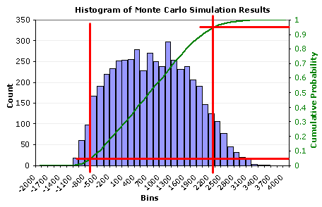
In Part 4 of this Monte Carlo Simulation example, we plotted the results as a histogram to visualize the uncertainty in profit. We are going to augment the histogram now by including a graph of the estimated cumulative distribution function (CDF) as shown below.
Download the Sales Forecast Example

Figure 1: Graph of the estimated cumulative distribution.
The reason for showing the CDF along with the histogram is to demonstrate that an estimate of the cumulative probability is simply the percentage of the data points to the left of the point of interest.
For example, we might want to know what percentage of the results was less than -$700.00 (the vertical red line on the left). From the graph, the corresponding cumulative probability is about 0.05 or 5%. Similarly, we can draw a line at $2300 and find that about 95% of the results are less than $2300.
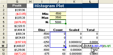
It is fairly simple to create the cumulative distribution in Excel. Figure 2 shows how you can estimate the CDF by calculating the probabilities using a cumulative sum of the count from the frequency function. You simply divide the cumulative sum by the total number of points.

Figure 2: Calculating the probabilities for the cumulative distribution.
Percentile and Rank Functions
Many of the questions we may have about the results of our simulation can be answered by using the CDF to go from a cumulative probability to a percentile or vice versa. The PERCENTRANK() and PERCENTILE() functions in Excel allow us to do this quite easily.
Note that a percentile, or quantile, refers to the value (in this case, the profit) corresponding to a given estimated cumulative probability.
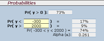
Question 1: What percentage of the results was less than -$700?
This question is answered using the percent rank function: =PERCENTRANK(array,x), where the array is the data range (column G in figure 2 above) and x is –$700.
If x matches one of the values in the array, this function is equivalent to the Excel formula =(RANK(x)-1)/(N-1) where N is the number of data points. If x does not match one of the values, then the PERCENTRANK function interpolates. You can read more about the details of the RANK, PERCENTILE, and PERCENTRANK functions in the Excel help file (F1).
The figure below shows a screen shot of some examples where the percent rank function is used to estimate the cumulative probability based upon results of the Monte Carlo simulation.

Figure 3: Calculating probabilities using the Excel percent rank function.
The accuracy of the result will depend upon the number of data points and how far out on the tails of the distribution you are (and of course on how realistic the model is, how well the input distributions represent the true uncertainty or variation, and how good the random number generator is). Recalculating the spreadsheet a few times by pressing F9 will give you an idea of how much the results may vary between each simulation.
Question 2: What are the 95% central interval limits? (alpha=0.05)
Stated another way: What are the 0.025 and 0.975 quantiles?
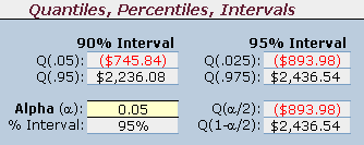
This is probably one of the most important questions, since the answer provides an important summary statistic that describes the spread of the data. The central interval is found by calculating the 0.025 and 0.975 quantiles, or Q(alpha/2) and Q(1-alpha/2), respectively.
The quantiles (or percentiles) are calculated by using the Excel percentile function: =PERCENTILE(array,p) where the array is the data range (column G) and p is the cumulative probability (0.025 or 0.975).
The figure below shows a screen shot of examples that use the percentile function in the Monte Carlo simulation example spreadsheet.

Figure 4: Calculating quantiles using the Excel percentile function.
Note that we are not using the term "confidence interval" to describe this interval. We are estimating what proportion of the data we expect to be within the given limits based upon the results of the simulation. We call it a central interval because we are defining the interval based upon the central proportion of the data.
The End
This concludes the Monte Carlo simulation example using Excel. This article is not comprehensive, and many details having to do with Monte Carlo simulation have not been covered. However, I hope this article has given you a good introduction to the basics.
REFERENCES:
- Vardeman, S.B., 1994, Statistics for Engineering Problem Solving, Boston: PWS Publishing Company. (pp. 66-69)
- PERCENTILE.EXC vs. PERCENTILE.INC at answers.microsoft.com
