PINTERP
=PINTERP(x, known_xs, known_ys, n)
| Argument | Description | Example |
|---|---|---|
| x | Value or vector of values to be interpolated | 2 |
| known_xs | Vector of known x values | {1;2;3;4;5} |
| known_ys | Vector of known y values | {0.9;0.14;-0.76} |
| n | Degree of the polynomial | 3 |
In the template file, navigate to the Polynomials worksheet to see the PINTERP function in action.
Description
PINTERP uses polynomial interpolation between the n+1 nearest points where n is the degree of the polynomial. The nearest points are found by first calculating the square of the distance from x as (x-xs)^2 for all points in known_xs. n+1 is the minimum number of points for exactly fitting a polynomial of degree n.
PINTERP uses the functions POLYVAL and POLYFIT on the subset of n+1 points to return the interpolated value.
The known (x,y) pairs do not need to be sorted because the function sorts the table after calculating the distances. x can be a single value or a vector.
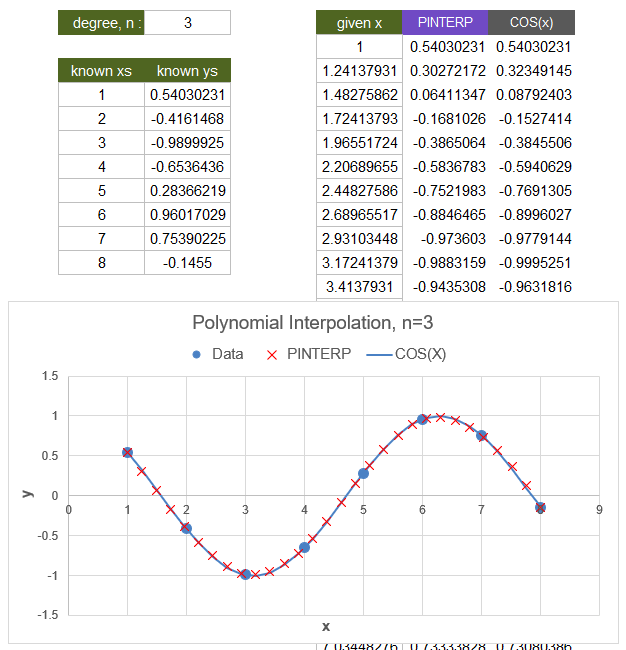
Polynomial interpolation and other types of interpolation can be useful for obtaining intermediate values when you only have a table of data rather than knowing the actual mathematical relationship between x and y.
For the sake of the following example, the known_ys values are calculated using COS(x). But, the purpose of interpolation is to find values based only on given data rather than knowing that actual formula for y.
COS(x) is shown in the example graph only to illustrate how closely the cubic (n=3) polynomial interpolation fits the actual curve.
Polynomial interpolation should not be confused with regression (statistically fitting a polynomial). If your data table contains statistical data with significant variation or scatter, polynomial interpolation may not be appropriate (see the example below). Linear regression tends to have a smoothing effect, but polynomial interpolation exactly fits a polynomial to the n+1 closest points.
Relationship to LINTERP
If n=1 (linear) and the two closest points are on either side of x, then PINTERP should return the same results as LINTERP. If x is not inbetween the two closest points, the results may differ from LINTERP.
Lambda Formula
This code for using PINTERP in Excel is provided under the License as part of the LAMBDA Library, but to use just this function, you may copy the following code directly into your spreadsheet.
Code to Create Function via the Name Manager
Name: PINTERP
Comment: Polynomial interpolation between the n+1 closest points
Refers To:

=LAMBDA(xs,known_xs,known_ys,n,
LET(doc,"https://www.vertex42.com/lambda/pinterp.html",
    xs,IF(AND(ROWS(xs)=1,COLUMNS(xs)>1),TRANSPOSE(xs),xs),
    known_xs,IF(AND(ROWS(known_xs)=1,COLUMNS(known_xs)>1),TRANSPOSE(known_xs),known_xs),
    known_ys,IF(AND(ROWS(known_ys)=1,COLUMNS(known_ys)>1),TRANSPOSE(known_ys),known_ys),
    BYROW(xs,LAMBDA(x,
        LET(tab,TAKE(SORT(HSTACK((known_xs-x)^2,known_xs,known_ys)),n+1),
            xo,INDEX(tab,1,2),
            POLYVAL(POLYFIT(INDEX(tab,0,2)-xo,INDEX(tab,0,3),n),x-xo)
        )
    ))
))
Code for AFE Workbook Module (Excel Labs Add-in)
/**
* Polynomial interpolation between the n+1 closest points based on distance (x0-x)^2
*/
PINTERP = LAMBDA(xs,known_xs,known_ys,n,
LET(doc,"https://www.vertex42.com/lambda/pinterp.html",
    xs,IF(AND(ROWS(xs)=1,COLUMNS(xs)>1),TRANSPOSE(xs),xs),
    known_xs,IF(AND(ROWS(known_xs)=1,COLUMNS(known_xs)>1),TRANSPOSE(known_xs),known_xs),
    known_ys,IF(AND(ROWS(known_ys)=1,COLUMNS(known_ys)>1),TRANSPOSE(known_ys),known_ys),
    BYROW(xs,LAMBDA(x,
        LET(tab,TAKE(SORT(HSTACK((known_xs-x)^2,known_xs,known_ys)),n+1),
            xo,INDEX(tab,1,2),
            POLYVAL(POLYFIT(INDEX(tab,0,2)-xo,INDEX(tab,0,3),n),x-xo)
        )
    ))
));
Named Function for Google Sheets
Name: PINTERP
Description: Polynomial interpolation between the n+1 closest points
Arguments: xs, known_xs, known_ys, n
Function:

LET(doc,"https://www.vertex42.com/lambda/pinterp.html",
    xs,IF(AND(ROWS(xs)=1,COLUMNS(xs)>1),TRANSPOSE(xs),xs),
    known_xs,IF(AND(ROWS(known_xs)=1,COLUMNS(known_xs)>1),TRANSPOSE(known_xs),known_xs),
    known_ys,IF(AND(ROWS(known_ys)=1,COLUMNS(known_ys)>1),TRANSPOSE(known_ys),known_ys),
    BYROW(xs,LAMBDA(x,
        LET(tab,CHOOSEROWS(SORT(HSTACK((known_xs-x)^2,known_xs,known_ys)),SEQUENCE(n+1)),
            xo,INDEX(tab,1,2),
            ARRAYFORMULA(POLYVAL(POLYFIT(INDEX(tab,0,2)-xo,INDEX(tab,0,3),n),x-xo))
        )
    ))
)
Google Sheets doesn't have a TAKE function, so the GS formula uses CHOOSEROWS.
PINTERP Examples
Test: Copy and Paste this LET function into a cell
=LET(
    x, LINSPACE(1,10,31),
    known_xs, LINSPACE(1,10,11),
    known_ys, RANDARRAY(11,1),
    n, 3,
    PINTERP(x,known_xs,known_ys,n)
)

Result: [variable because of RAND]
Using polynomial interpolation generally assumes that function is continuous but unknown. The actual data in this case, being random, would definitely not follow the pattern assumed by the interpolated points. Be careful when using interpolation with random or scattered data.
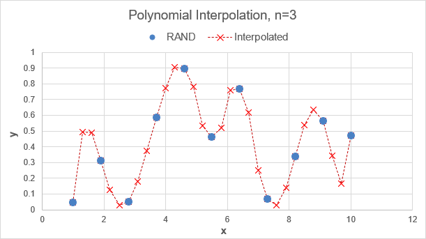
On the other hand, if this sample data did truly represent a continuous curve, then you can see how polynomial interpolation might approximate values between the various points. Cubic polynomial interpolation (n=3) uses only the 4 nearest points, so the the result is very different from using a single cubic polynomial fit of the entire data set.
Test: Copy and Paste this LET function into a cell
=LET(
    n, 3,
    xs, LINSPACE(1000,1000+PI(),n+1),
    ys, COS(xs),
    POLYVAL(POLYFIT(xs,ys,n),xs)
)

xs: {1000; 1001.047; 1002.094; 1003.142}
ys: {0.562; -0.435; -0.997; -0.562}
Result:
yp: {0.59;  -0.519; -0.913; -0.59}
yp are the values returned from POLYVAL(POLYFIT()) and they should be exactly the same as ys. To help reduce this problem, we can introduce a shift in the x values prior to doing the fit, which is the same thing we do with piecewise polynomials. This shifts the curve to start at x=0 prior to fitting:
Test: Copy and Paste this LET function into a cell
=LET(
    n, 3,
    xs, LINSPACE(1000,1000+2*PI(),n+1),
    xo,INDEX(xs,1),
    ys, COS(xs),
    POLYVAL(POLYFIT(xs-xo,ys,n),xs-xo)
)

Result: {0.562;-0.435;-0.997;-0.562}
This example demonstrated the error using POLYVAL(POLYFIT()) because this same procedure is used within PINTERP. PINTERP has been updated with the shift in x as of version 1.0.7 of the lambda library.
See Also
SE, LINSPACE, LINTERP, PPVAL, POLYDER
Revision History
- 3/7/2024: Added the xo shift to improve numeric stability at large values of x
