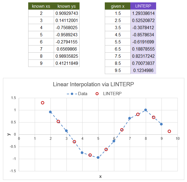
LINTERP - Linear Interpolation Function for Excel

=LINTERP(x, known_xs, known_ys)

Argument	Description	Example
x	Value or vector of values to be interpolated	2
known_xs	The known x values	{2;3;4}
known_ys	The corresponding known y values	{0.9;0.14;-0.76}

Download the Template

In the template file, navigate to the Polynomials worksheet to see the LINTERP function in action.

Description

LINTERP uses linear interpolation between the two nearest points in a table lookup to return the value y for a given x. If the value for x is outside the domain of known xs, then the point is extrapolated from the closest two data points (either the first or last 2 points).

The known (x,y) pairs do not need to be sorted because the function sorts the points prior to doing the table lookup. x can be a vector of x values or a single value.

Linear Interpolation Formula

Linear interpolation is used to calculate the position of a point on a line from two other known points on that line. A line is defined by two points: (x₁,y₁) and (x₂,y₂). Linear interpolation calculates a y₀ value for a known x₀ value using the formula:

$$y_0 = y_1+(x_0-x_1)\frac{y_2-y_1}{x_2-x_1}$$

Using spreadsheet-based formulas, you can linearly interpolate to find y0 for a given x0 using one of the following formulas (replacing xi and yi variables with cell references):

y0 = y1+(x0-x1)*(y2-y1)/(x2-x1)

y0 = SLOPE({y1;y2},{x1;x2})*x0+INTERCEPT({y1;y2},{x2;x2})

y0 = FORECAST.LINEAR(x0,known_ys,known_xs)

Interpolating from a table of data is more of a challenge (involving table lookups), which is why the LINTERP function is easier to use.

Note: Using FORECAST.LINEAR works when you only have two points. However, if you try to use it the same way a LINTERP you will get a different answer because FORECAST.LINEAR fits a line to the entire set of points (using regression) instead of doing a table lookup to find just the 2 closest points.

Lambda Formula

This code for using LINTERP in Excel is provided under the License as part of the LAMBDA Library, but to use just this function, you may copy the following code directly into your spreadsheet.

Code to Create Function via the Name Manager

Name: LINTERP
Comment: Linearly interpolate between the two nearest points in Excel
Refers To:

=LET(doc,"https://www.vertex42.com/lambda/linterp.html",
    xs,IF(AND(ROWS(xs)=1,COLUMNS(xs)>1),TRANSPOSE(xs),xs),
    known_xs,IF(AND(ROWS(known_xs)=1,COLUMNS(known_xs)>1),TRANSPOSE(known_xs),known_xs),
    known_ys,IF(AND(ROWS(known_ys)=1,COLUMNS(known_ys)>1),TRANSPOSE(known_ys),known_ys),
    tab,SORT(HSTACK(known_xs,known_ys)),
    BYROW(xs,LAMBDA(x,
        LET(ind,MATCH(x,INDEX(tab,0,1),1),
            pts,
            IF(x<=MIN(known_xs),TAKE(tab,2),
                IF(x>=MAX(known_xs),TAKE(tab,-2),
                    CHOOSEROWS(tab,ind,ind+1)
                )
            ),
            SLOPE(INDEX(pts,,2),INDEX(pts,,1))*x+INTERCEPT(INDEX(pts,,2),INDEX(pts,,1))
        )
    ))
));

Code for AFE Workbook Module (Excel Labs Add-in)

/**
* Linearly interpolate between the two nearest points in a table lookup
*/
LINTERP = LAMBDA(xs,known_xs,known_ys,
LET(doc,"https://www.vertex42.com/lambda/linterp.html",
    xs,IF(AND(ROWS(xs)=1,COLUMNS(xs)>1),TRANSPOSE(xs),xs),
    known_xs,IF(AND(ROWS(known_xs)=1,COLUMNS(known_xs)>1),TRANSPOSE(known_xs),known_xs),
    known_ys,IF(AND(ROWS(known_ys)=1,COLUMNS(known_ys)>1),TRANSPOSE(known_ys),known_ys),
    tab,SORT(HSTACK(known_xs,known_ys)),
    BYROW(xs,LAMBDA(x,
        LET(ind,MATCH(x,INDEX(tab,0,1),1),
            pts,
            IF(x<=MIN(known_xs),TAKE(tab,2),
                IF(x>=MAX(known_xs),TAKE(tab,-2),
                    CHOOSEROWS(tab,ind,ind+1)
                )
            ),
            SLOPE(INDEX(pts,,2),INDEX(pts,,1))*x+INTERCEPT(INDEX(pts,,2),INDEX(pts,,1))
        )
    ))
));

Named Function for Google Sheets

Name: LINTERP
Description: Linearly interpolate between the two nearest points in Excel
Arguments: xs, known_xs, known_ys
Function:

LET(doc,"https://www.vertex42.com/lambda/linterp.html",
    xs,IF(AND(ROWS(xs)=1,COLUMNS(xs)>1),TRANSPOSE(xs),xs),
    known_xs,IF(AND(ROWS(known_xs)=1,COLUMNS(known_xs)>1),TRANSPOSE(known_xs),known_xs),
    known_ys,IF(AND(ROWS(known_ys)=1,COLUMNS(known_ys)>1),TRANSPOSE(known_ys),known_ys),
    tab,SORT(HSTACK(known_xs,known_ys)),
    BYROW(xs,LAMBDA(x,
        LET(pts,
            IF(x<=MIN(known_xs),CHOOSEROWS(tab,{1;2}),
                IF(x>=MAX(known_xs),CHOOSEROWS(tab,{ROWS(tab)-1;ROWS(tab)}),
                    CHOOSEROWS(tab,SEQUENCE(2,,MATCH(x,INDEX(tab,0,1),1)))
                )
            ),
            SLOPE(INDEX(pts,0,2),INDEX(pts,0,1))*x+INTERCEPT(INDEX(pts,0,2),INDEX(pts,0,1))
        )
    ))
)

Google Sheets doesn't have a TAKE function (yet?), so the GS function uses CHOOSEROWS instead.

Warning

These functions are not compatible between Excel and Google Sheets. When using these functions, you will not be able to convert the Excel file to Google Sheets or vice versa without problems.

LINTERP Examples

Example 1

Generate the values shown in the example image above.

Test: Copy and Paste this LET function into a cell
=LET(
    xs, LINSPACE(1.5,9.5,9),
    known_xs, SE(2,9),
    known_ys, SIN(known_xs),
    LINTERP(xs,known_xs,known_ys)
)

Result: {1.293;0.525;-0.308;-0.858;-0.619;0.189;0.823;0.701;0.123}

Example 2

A line is defined by two points (x1,y1)=(2,3) and (x2,y2)=(4,2.5). Find the y value for the point where x=3.

Test: Copy and Paste this LET function into a cell
=LET(
    x, 3,
    known_xs, {2;4},
    known_ys, {3;2.5},
    LINTERP(x,known_xs,known_ys)
)

Result: 2.75

LINTERP - Linear Interpolation Function