2-Column Phone List Template
Printed phone directories and other types of narrow lists are typically printed in multiple columns either on a single page or multiple pages. Even though Excel is a great place to create and store lists, it doesn't have a print or page layout option for printing a long list in multiple columns automatically.
Some people use the solution of copying/pasting a list into Word and then formatting word to print multiple columns. That's an okay solution if you just need to do it once, or if your list is extremely long. But, if you are wondering how to set up a sortable 2-column list in Excel, download the phone directory template and continue reading below to learn how it was made.
This Page (contents):
Phone List Template
for Excel
Download
⤓ Excel (.xlsx)License: Private Use (not for distribution or resale)
Description
This template demonstrates how to create a 2-column list that uses Excel formulas to reference a data source. When the data source is sorted and/or filtered, the list updates automatically.
How to Create a Sortable 2-Column List in Excel
I created this template to answer a question posed to me by Jonathan Weinraub about how to make a sortable 2-column phone directory. The problems were how to make the directory update automatically when the data source was sorted, and how to prevent #REF! errors when rows were deleted from the data source.
Step 1: Create the Data worksheet
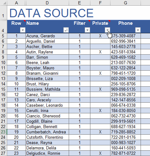
Our data source is a separate worksheet with an Excel Table consisting of names, phone numbers, and other contact information (created using the Contact List Template).
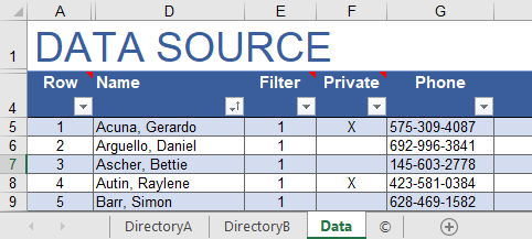
The contact list can be formatted as an Excel Table by going to Home > Format as Table. This is a special feature in Excel that allows you to use structured refences. I've named the Table "ContactList" via Formulas > Name Manager.
Step 2: Create a separate Phone Directory worksheet
The Directory worksheet will be used for printing the multiple-column phone list, so create it using whatever formatting, fonts and colors you want.
Step 2a: Create groups of columns for Row #, Name, and Phone
As demonstrated in the phone list template, I have 2 separate groups of columns labeled #, Name, Phone. The # column is critical - it will be used to reference the corresponding row from the Data worksheet.
Note: Before printing, the # columns can be hidden if you don't want them shown.
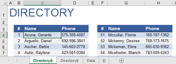
The first # column is numbered 1 through 50, and the second is numbered 51 through 100. You can manually enter the numbers, or in cell B5 enter the formula =B4+1 or =OFFSET(B5,-1,0) and copy the formula down to fill in the # column. The top value in the # column can reference the last cell in the previous # column, plus 1.
Using OFFSET or a relative named range (like =cellAbove+1) to reference the value 1 cell above the current cell allows you to insert and delete rows without messing up the numbering. See the article "Create a Running Balance in Excel that Allows you to Insert, Delete, and Move Rows" to learn more about this technique.
Step 2b: Use the OFFSET function to look up the Name and Phone
The OFFSET(reference, offset_rows, offset_columns) function provides a powerful way to reference another cell. Using OFFSET to populate the Directory worksheet allows you to sort the Data worksheet and even insert and remove rows, without causing #REF! errors in the Directory.
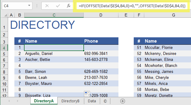
The formula for displaying the Name in cell C4 is =OFFSET(Data!$D$4,B4,0). Cell B4 = 1, so this formula references the cell that is 1 row below cell $D$4 in the Data worksheet.
Copy the formula down to fill in the Name column in the directory, then do the same thing for the Phone column (using Data!$G$4 as the reference cell).
Note: The template uses structured references, so instead of Data!$D$4, the reference to the header of the Name column is ContactList[[#Headers],[Name]]. Either way works.
Step 3: Format Tricks for the Directory
In the directory worksheets, I used conditional formatting to highlight every other row, because I am not using Excel Tables there.
To hide the zeros when the OFFSET function refers to a blank cell, I'm using a custom number format of 0;0;;@.
Step 4: Copy/Paste if you need Multiple Pages
This is the part that could get tedious if you have a really long list, or a list that frequently changes and varies in length. To create a new page below the first one, copy the entire group of rows you created in steps 1-3 and paste them below. Make sure to update the # columns as needed.
What if You Want to Filter the Contact List?
Excel's Data > Filter feature provides a simple way to quickly hide rows from a table or list.
For example, the template includes a column labeled "Private" that can be used for marking contacts that you don't want to display in a printed phone list. The animated image below shows how to hide the rows marked with an "X" and then how to clear the filter.
When you use the filter feature in the Data worksheet to hide rows, the OFFSET function in the Directory will still display the hidden names. So, to create a formula that skips the hidden rows, we first need a formula that can tell us when a row is hidden.
How do you detect if a row is hidden?
The SUBTOTAL function can be used to sum and count values, ignoring hidden cells, so we can use SUBTOTAL to detect if a row is hidden. The Filter column in our Contact List table uses the formula =SUBTOTAL(103,[@Name]). The 103 value tells SUBTOTAL to use the COUNTA function to only count cells that are not hidden (and all we are doing is counting a single cell). The structured reference, [@Name], is referencing the cell in the Name column that is on the same row as the cell containing the formula.
You can't see it, but the value in the Filter column is zero (0) in the hidden rows. That is because the count returned by SUBTOTAL will be 0 for those cells.
Returning to the DirectoryA worksheet, we can use an IF function to display a blank if the Filter value is zero. See the formula for cell C4 in the image below.
You may not want your directory full of blank rows where the data source has been filtered. In that case, continue reading.
How can we skip filtered rows rather than showing them as blanks?
For this technique, you can use an INDEX-MATCH lookup formula instead of the OFFSET function. That is why the Data worksheet has a Row column.
First, in the Data worksheet, use the SUBTOTAL function in the Row column to create a running count of just the non-hidden rows. The formula in cell A5 is =SUBTOTAL(103,$D$4:D5)-1, and that formula is copied down to fill in the data table.
Look back at the animated gif above and notice what happens in the Row column when the list is filtered. The hidden rows are not counted, so you should see that the Row column appears to stay the same even though some rows are hidden.
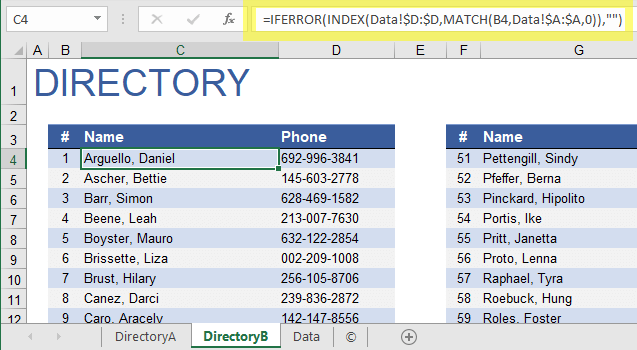
Next, returning to the DirectoryB worksheet, use an INDEX-MATCH function to return the Name by looking up the row number as shown in the image below. Note: The IFERROR function surrounding the formula is used to display a blank when no match is found.
So, there you have it. We've created a 2-column phone list that lets you sort and filter the source table. You can also insert and delete rows in the source table without causing #REF! errors in the directory.
