In Excel, you aren't limited to using built-in number formats. You can define your own custom number formats to display values as thousands or millions (23K or 95.3M), add leading zeros, display " - " for zero values, make negative values red, add bullets, and much more.
This Article (bookmarks):
Watch the video we created to go along with this article!
How to Create a Custom Number Format
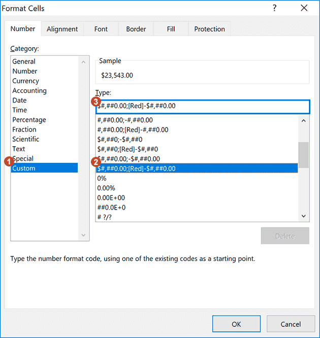
To create a custom number format, it is easiest to begin with a built-in format. Open the Format Cells dialog box by pressing Ctrl+1 (or right-click on a cell and select Format Cells) and select the Number tab (see the image below). Then (1) Choose Custom from the Category list, (2) Select a built-in format similar to what you want, and (3) Edit the format string in the Type field.
Number Format Codes
A number format string uses up to 4 different codes, separated by semicolons, as shown in the image below.
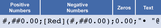
Instead of explaining the syntax in detail at this point, let's take a look at some examples and learn as we go.
Some of the characters like #, 0, @, etc. have special meanings. Some codes like [Red] can change the font color, and quotes can be used to display text or special characters. The table below summarizes some of these special characters.
Special Characters in Number Formats
| Character | Description |
|---|---|
| # | A digit placeholder |
| 0 | A digit that is to be displayed even if it is zero |
| , | (Comma) Interpreted as a 1000's marker |
| @ | Represents the value displayed as text |
| * | (Asterisk) Repeats the next character to fill the cell |
| [ColorCode] | See the section below about using color codes |
| [<=100] | Conditional operators (valid only in the Positive and Negative sections) |
| / | Used for fractions such as # #/12 or as the / character for dates |
| " " | (Quotes) Used to display whatever is contained within the quotes as text, such as 0.00 "feet" |
| d or dd ddd dddd |
Day number (0-31 or 00-31) Abbreviated day of week (Mon, Tue, etc.) Full day of week (Monday, Tuesday, etc.) |
| m or mm mmm mmmm mmmmm |
Month number (0-12 or 00-12) Abbreviated month name (Jan, Feb, etc.) Full month name (January, February, etc.) First letter of the month (J, F, M, etc.) |
| y or yy yyyy |
Year (0-99 or 00-99) Full year (1900-9999) |
| h or hh m or mm s or ss |
Hour (0-23 or 00-23) Minutes (0-59 or 00-59) Seconds (0-59 or 00-59) |
NOTE Some characters are specific to locale/language settings. For example J is used for Year in some countries.
Custom Number Format Examples
The examples below show some of the custom number formats that I've found the most useful. This isn't a comprehensive list of all possible number formats. See support.microsoft.com to search for other articles on this subject.
TIP Using a custom number format only affects the displayed value. A formula that references the cell will use the stored value no matter how it is displayed. This means you can still use a formula to refer to the value even though the number might be displayed as "12 ft."
To see these examples in action, download the Excel file below.
Download the Example File (CustomNumberFormats.xlsx)
Custom Number Format for Thousands and Millions
| Format Code | Value | Displayed As | Description |
|---|---|---|---|
| 0,K 0.0,K 0.0, "Thousand" |
23543 | 24K 23.5K 23.5 Thousand |
Display values in thousands, using the letter K to indicate thousands. The "K" is just a displayed character - it has no special meaning in the number format string. If you want to display more than one letter, you need to enclose the characters in quotes, like the "Thousand" example. |
| 0,,"M" 0.0,,"M" 0.0,, "Million" |
23543000 | 24M 23.5M 23.5 Million |
Display values in millons, using the letter M to indicate millions. Note that in this case, you need two commas. |
NOTE These are very useful for chart axes and labels.
Display Leading Zeros and Include Commas
| Format Code | Value | Displayed As | Description |
|---|---|---|---|
| 000 00000 |
50.8 | 051 00051 |
Display values with leading zeros. This does not convert the value to text - it is only a display format. |
| #,##0.0 | 3543.46 | 3,543.5 | Display values using commas to separate thousands, millions, etc. The # sign is used as a placeholder, meaning that if there are no 10's, 100's, or 1000's, don't display them. |
Display Units Without Converting to Text
| Format Code | Value | Displayed As |
|---|---|---|
| • Display a number and text in the same cell using the conditions [=1] and [>1]. The value is stored as a number, so you can still do calculations on the number of people. | ||
| [=1]# "person";[>1]# "people";0 | 1 5 0 |
1 person 5 people 0 |
| • Display a number and text in the same cell. The value is stored as a number, so you can still do calculations. | ||
| 0.0 "ft" 0.0 "kg" # #/## "in" |
2.2 4.5 6.25 |
2.2 ft 4.5 kg 6 1/4 in |
| • Display a numeric YYMMDD value in years, months, days. | ||
| ##"y" ##"m" ##"d" | 360712 | 36y 07m 12d |
Special Time Formats
There are quite a few built-in time formats to choose from. The following may be less known.
| Format Code | Value | Displayed As | Description |
|---|---|---|---|
| [h]:mm:ss [h]:mm [mm]:ss [ss] |
49:03:47 | 49:03:47 49:03 2943:47 176627 |
Shows elapsed time in hours, minutes or seconds. Note that time does not round up. |
| h:mm A/P h:mm a/p |
2:25 PM | 2:25 P 2:25 p |
Displays time using "a" for AM and "p" for PM. Useful when trying to minimize column widths without making fonts smaller. |
Including Special Symbols
Some ascii and unicode characters can be copied and pasted directly into the format code. This can be handy for displaying the degrees symbol for temperatures as well as other tricks like showing up and down arrows or bulleted lists.
| Format Code | Value | Displayed As | Description |
|---|---|---|---|
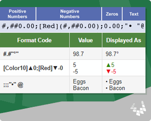
| #.#"°" | 98.7 | 98.7° | Display temperature in degrees with the ° symbol. |
| [Color10]▲0;[Red]▼-0 | 5 -5 |
▲5 ▼-5 |
Display special symbols for positive and negative, combined with colors. |
| ;;;"•" @ | Eggs Bacon |
• Eggs • Bacon |
Create a bulleted list using a special symbol for the bullet. When you enter text, the bullet will be displayed. Numbers and zero values will not be displayed. |
NOTE You can also include unicode characters like ✔ or 😁. See the article "Using Unicode Character Symbols in Excel" for a list of useful symbols.
Displaying Fractions
| Format Code | Value | Displayed As | Description |
|---|---|---|---|
| # ??/12 | 5.75 12.5 |
5 9/12 12 6/12 |
Display a decimal number of feet as feet and inches (rounded to the nearest inch). Or display a decimal year in terms of years and months. |
| # ??/100 | 5.2 5.05 12.81 |
5 20/100 5 5/100 12 81/100 |
Using ??/100 will help line up values in a column (as opposed to just using ?/100). Note that fractions are automatically rounded. |
| ?/2 | 5.2 | 10/2 | Displays a simple fraction as numerator/denominator. |
Trailing and Leading Characters to Fill a Cell
The asterisk (*) in a format code repeats the following character to fill the width of the cell.
| Format Code | Value | Displayed As | Description |
|---|---|---|---|
| -- @ *- | ✁ | -- ✁ ---------------- | Trailing characters. |
| *.@ | pg 2 | ..................pg 2 | Leading characters |
Custom Number Formats for Chart Axes and Labels
| Format Code | Value | Displayed As | Description |
|---|---|---|---|
| 0 "AD";0 "BC" | 247 -600 |
247 AD 600 BC |
AD and BC Years. Use negative numbers for BC years and positive numbers for AD years. |
| mmm{Ctrl+j}yyyy | 8/20/18 | Aug 2018 |
Add a Carriage Return within the custom number format (e.g. between dddd and mmm) by pressing Ctrl+j. |
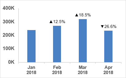
| [Color10]▲0.0%;[Red]▼-0.0% | 15.23% -23.57% |
▲15.2% ▼-23.6% |
Display arrows for positive and negative, combined with colors and percentages. |
A couple of these examples can be seen in the image below. However, notice that the data labels don't use color codes, so the percentages are shown only as black text rather than red and green. Too bad. Maybe Microsoft will fix that some day.
NOTE Editing a custom number format that contains a carriage return is tricky because you can't see the second row. This is why I write out the code first using "{Ctrl+j}" or just "{j}" and then delete the "{j}" and press Ctrl+j in its place.
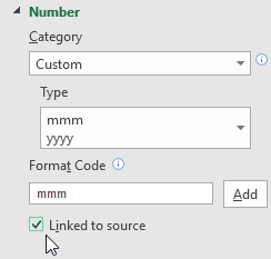
When adding a custom number format using the Format Axis window pane, you may not be able to press Ctrl+j to add a carriage return. In that case, first edit the format of the data source, then click on the Link to Source box as shown in the image to the right. After doing that, you can uncheck the Link to Source box and modify the original data source formatting.
Other Tricks
| Format Code | Value | Displayed As | Description |
|---|---|---|---|
| ;;; | anything | Display nothing, regardless of the value. | |
| 0.# | 2 | 2. | Display a decimal point without a 0 after the decimal (2. instead of 2.0) |
| ???.??? | 1.2 12.3 123.456 |
1.2 12.3 123.456 |
Vertically align the decimal point when displaying a column of numbers. |
NOTE If you are looking for format codes for phone numbers, social security numbers, or zip codes, look in the Special category within the list of built-in number formats.
Custom Number Format Color Codes
By using color format codes such as [Red] or [Blue] or [Color10], you have a limited ability to alter the color of the font via custom number formats. The most common use I've seen is to color negative values red. However, one of the examples above also shows how you might want to use a green arrow.
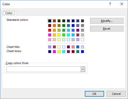
Even though a new color palette was introduced in Excel 2007, the color codes for custom number formats are still based on the old color palette for the Excel 97-2003 format. I created the graphic below to provide a quick reference.

I made the above color code reference match the layout of the old color palette because there is not a consistent pattern to the numbering.
Define Your Own Color: You can modify the color palette in newer versions of Excel by going to File > Options > Save > Colors. This allows you to change the color associated with the Color1 through Color56 codes. This means that Color10 might not always be a dark green. If you purposely change the color palette (or somebody else does), Color10 might be some other color.
Excel 2016: File > Options > Save > Colors
NOTE The Color1-56 codes in Google Sheets are fixed colors and aren't changed when you upload an Excel file with a customized color palette.
Conditional Operators
Conditional operators such as [<100] can be used to change the formatting in cases where positive;negative;0 is not how you want the divisions defined.
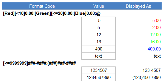
For example, the following format will display numbers less than 10 red, numbers between 10 and 20 green, other numbers blue, and text will be displayed based on the cell's font color: [Red][<10]0.00;[Green][<=20]0.00;[Blue]0.00;@
You are limited to 2 numeric conditions, which you place in the negative and positive sections of the format code.
Another use of conditional operators is to display phone numbers with and without an area code, depending on how many digits are in the phone number like this: [<=9999999]###-####;(###)###-####. This assumes that the phone numbers are entered as numbers and not text values. Meaning, that if you actually enter 123-1234 into a cell in Excel, it will be interpreted as a text value, not a number. The phone number format will display 1234567 to 123-4567 and it will display 1234567890 to (123)456-7890.
Custom Location Codes for Dates
When displaying month names and weekday names for dates, you can use location codes such as [$-fr-CA] at the beginning of the format code to tell Excel to display the names in other languages. To learn what the code is for a specific language and location, use the Format Cells dialog in Excel, choose one of the built-in Date formats, then choose the Locale (location) from the drop-down list. Then you can return to the Format Cells dialog box and click on the Custom tab to see what location code was added.
| Format Code | Value | Displayed As | Language/Location |
|---|---|---|---|
| [$-en-US](ddd) mmm d, yyyy | 10/1/2018 | (Mon) Oct 1, 2018 | English (United States) |
| [$-fr-CA](ddd) mmm d, yyyy | 8/1/2018 | (mer.) août 1, 2018 | French (Canada) |
| [$-de-DE](ddd) mmm d, yyyy | 10/1/2018 | (Mo) Okt 1, 2018 | German (Germany) |
Other Notes About Custom Number Formats
To delete a custom number format, open the Format Cells dialog box, select the custom format from the list, then click Delete. When you delete a custom number format, all values in your workbook that use that format will revert to the General format.
Custom number formats that you create are saved with the file. If you want to use the custom format in a different file, you can copy/paste the formatting from your other file by copying and pasting the formatted cell or using the Format Painter tool.
References
- Number Formats for Charts by Jon Peltier, Excel MVP
- Excel Custom Number Format Guide by Mynda Treacy, Excel MVP


Comments
Conditional Operators: We can use comma separator with format shown above:
[Red][<10]###,##0.00;[Color10][<=5000]###,##0.00;[Blue]###,##0.00;@
A great help in visually separating entries using colour code.
Wonderful article! We will be linking to this particularly great article on our site. Keep up the good writing.
We appreciate you sharing this info with this awesome web site. let me promote the next few paragraphs in my zynga be the cause of my friends
Major thanks for the blog post. Want more.
great summary … first place I have found that clarifies the process of entering a line break into a format of a chart axis … too bad it has to be this complicated
Very interestiing article
I would like (and I will pay if necessary) to know how to create a format that in negative numbers places the – signus by the number
For instance, I hace created a format to express errors in mm. “E=”0,0″mm”
The problem comes when the number is negative, this is -1.3 is formated as -E=1.3mm
Is there any way to get E=-1.3mm
Looking forward to receiving your comments and thanking you in advance
Best regards
Sure, just use the 2nd part of the conditional formatting code to specify exactly how you want the negative format to appear: “E=”0.0″mm”;”E=-“0.0″mm”
Is there a way to not round a number in the custom format
@Julie … good question, but I don’t think so. Excel will always display only a specific number of decimal places based either on the format you choose, or if it’s a General format based on the width of the cell. I could be wrong though and would be interested if there was a way to make Excel stop rounding numbers when displayed.
Thank you for this guide! I finally understand how to use the semicolon to separate different formats for positive and negative numbers. This will save me a lot of time on my monthly reports.