
In December, 2020 we released a new version of Gantt Chart Template Pro that is designed to consolidate multiple versions and features into a single template. It is available to both new and current customers. Existing customers can return to the download page to get the new version (no new purchase necessary).
When I first created the Gantt chart template for Excel, my goal was simplicity and ease-of-use with minimal learning curve. Over time it became more complex as people requested new features, capabilities, and different ways to define task durations and dependencies. As with version 4.0, my goal for this new version was to maintain the idea of "Gantt Charts Made Easy!" while still providing as many awesome features as possible.
This page discusses some of the new features that were added or changed in Version 4.0 and 5.0.
This Page (contents):
1. WBS Numbering Controlled with a Simple Drop-Down Selection
You don't need to understand how the formula works for the work breakdown structure (WBS) numbering (2.4, 3.1, 3.1.1, 3.1.2, etc.). All you need to do is select the WBS Level from a drop-down box. The WBS numbering is automatic. Also, the task descriptions are automatically indented based on the chosen WBS level.
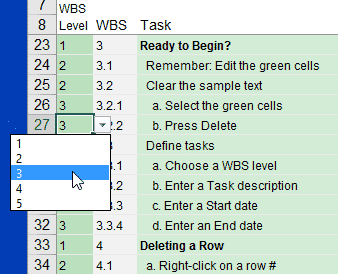
WBS Numbering via Drop-Down
Unlike the free version (and older pro versions), you will not need to copy and paste different WBS formulas for different WBS levels.
For fellow Excel fans: If you are curious about how the mega-formula for the WBS numbering works, you can learn some of the techniques via an article I wrote about various text manipulation formulas. Also, the indenting of the task description is controlled using Conditional Formatting and custom Number formats such as "_s_s_s_s@" to format the text with leading spaces.
2. Multiple Ways to Define Task Dates and Durations
The biggest change in version 4.0 had to do with how you define each task's start and end date. Instead of copying formulas from a set of template rows or cells to define tasks in different ways, you just enter your data in the appropriate input columns.
Watch the Video for Version 5.0
Ultimately, a task needs to have a start date and an end date. You can arrive at those dates in a lot of different ways, depending on whether you want to enter dates manually, enter a duration instead of a date, or whether you want to create dependencies between tasks using Excel formulas.
Now, all you need to do is enter a combination of two inputs. For example, this could be the Start date and End date, or the Start date and number of Work Days. The worksheet has separate columns for the calculated start & end dates. These calculated Start and End dates are what the spreadsheet uses to display the chart.
The downside to this new way of defining tasks is that there are quite a few input columns as well as the calculated columns. However, after you are done defining your tasks, you could hide some or all of the columns you don't need to see.
Tip: In addition to hiding columns to condense the input section of the worksheet, you can use the Arial Narrow font and then make the columns narrower.
Update 12/1/2021: There is now a new Lead/Lag column hidden right after the Predecessors columns. Using this optional column will make the task start X work days after (Lead) or before (Lag) the end date of the predecessor. Enter a positive value for Lead or a negative value for Lag. This column only works in combination with the Predecessors column.
3. Compatibility with Desktop, Mobile and Excel Online
Many of the design aspects of Version 5.0 have to do with making the spreadsheet compatible with Excel Online and Excel Mobile without having to use different versions of the file for different versions of Excel. The spreadsheet uses some features of Excel that are not available in Excel Online such as cross-hatching for displaying Actual vs. Planned - but the spreadsheet also includes a way to make this work in Excel Online (see the help and labels and notes within the spreadsheet).
Questions?
If you have questions about Gantt Chart Pro, please first watch the videos available on the web page, then check the Help worksheet, and then check the FAQ post. If you still can't find the answer to your question, you can contact me.
Q. Why are there two sets of Start/End dates?
The input columns allow you to quickly decide whether to enter dates and/or durations. However, the Gantt chart needs to reference a single column for all Start Dates and a single column for all End Dates. So, the calculated columns use formulas to calculate the dates based on which combination of inputs you choose, and the Gantt chart references these calculated columns.
When printing or presenting, it is better to hide the input columns instead of the calculated columns, because the calculated columns show ALL dates and durations while the inputs may or may not be used. For example, you might define a task by entering a Predecessor and a duration in Days, which means the inputs for Start date and End date are left blank.
Q. Is there any reason to use the older version(s)?
I don't think so, unless you are using an old version of Excel, or you prefer the older designs. However, the older versions will not be updated or supported.
Q. Why are some videos still showing the older versions?
Some older videos are still lingering on Youtube and elsewhere, and for the most part these older videos are still mostly applicable to the new version. See the Gantt Chart Pro page for the most recent videos.
Q. What happens if I enter more than two values to define task durations?
Avoid doing that. If you enter a Start Date and an End Date AND the number of Work Days, then you won't know which of the 3 values were used to calculate the Start and End dates used in the chart.
Q. What is happening when I enter End Date and Work Days as the inputs?
The Start date is calculated to be the number of work days PRIOR to the End date you entered. You might use this for a task that needs to start 5 days prior to the completion of some other task. The End date could be a simple Excel formula that references the end date of the other task.
Q. How do I work backwards from a known project end date, using dependencies?
Version 5.0 allows you to define a task using an End Date and the Duration (in days or work days). You'll just need to enter a formula in the End Date input column such as this one: =WORKDAY.INTL(successor_start_date,-1,weekend,holidays). See the Help worksheet for examples of using formulas to create task dependencies.
Q. What are the little green triangles in some of the cells?
The green triangles are due to the "Error Checking" feature in Excel. Most of the time they aren't actually errors. They may be warnings such as "Number stored as text" or "Inconsistent Formula" or "Unprotected Formula," all of which may be intentional on the part of the user or template designer (such as the WBS numbering purposefully entered as text).
To get rid of the green triangles, you can either choose the "Ignore Error" option every time they show up, or you can go to "Error Checking Options" to turn off some of the various types of warnings.
Q. Will the BONUS files be updated, too?
Perhaps. I've updated the Google Sheets version to 5.0, and will eventually update the other bonus files. However, I do not have a schedule for when that might happen.
Q. How do I show the overall % Complete for the entire project?
The latest update (5.0.1) includes a cell above the % Done column showing the progress for the entire project. If you aren't using the latest version and you want to add this formula to your spreadsheet, you can use the following formula (this requires Excel 2013 or later because of the ISFORMULA function). Note that this formula allows you to ignore the cells in the progress_range that contain formulas, such as if you are calculating the % Done for summary tasks (your overall % Done should not double count the summary tasks rows).
=SUMPRODUCT(workdays_range,progress_range,1*NOT(ISFORMULA(progress_range)))/SUMPRODUCT(workdays_range,1*NOT(ISFORMULA(progress_range)))


Comments
I’m looking forward to trying the new WBS numbering tool – that had me flummoxed in the current version! Thanks for this.
Hi John,
Both the Desktop and Mobile versions seem to be exactly the same (i.e. the file names are exactly identical and work both on the full version of Excel 2013 and also the Office 365 version) so not sure why there is a need to have two different downloads(?)
–YS
@Yogesh, Thanks for catching that. I’ve fixed the second link.
Hi Jon,
First of all – thanks for all the nice work- highly appreciated. Now i have a feature request: how do i create multiple dependencies in the Gantt v4 version? While creating this by myself was not a problem in the v3 version, the v4 version is given a lot of problems . Any indication whether we might expect his feature please?
Thanks and best regards,
P.
@Pascal… Due to multiple requests, I’ve updated version 4 with 2 more Predecessor columns (you can download the new files by returning to the download page). Two of the columns are hidden by default, so if you want to define up to 3 predecessors for a task, you can unhide these other predecessor columns.
Jon,
Fantastic & thank you very much!!!
Best regards,
Pascal
[Referring to the Google Sheets version]
Hello, I have noticed the following:
– in the weekly view
– when an action spans more than two weeks
– if the action is marked 100% complete
– then the last column of the line in the chart appears “in progress” (blue) instead of gray as are all the previous columns.
This does not happen in daily view.
Other than that, it’s an amazing piece of work, thank you very much.
This is great! There are just a couple things that I would love to bring into the new version from the older one.
– Is there a way to break the week cells into smaller bars to indicate which day on the graph like the old version showed? It seems like you would need to add more columns, but I’m not sure what the formula would need to be in Row 4.
– Is there an easy way to get a Planned vs. Actual bar format into this version?
Thanks so much!
@Amy … The file gantt-chart_v4-0.xlsx still uses more columns (7 columns per week in the weekly view) to display the gantt chart. The “o365” version was designed for compatibility with the online Excel app so fewer columns were used to reduce the computation power required (i.e. fewer formulas).
– Although the gantt chart doesn’t show planned vs. actual, you could insert two new Start and End date columns for storing the original planned time frame. I’ll consider adding a planned vs. actual version (like the old beta trial).
Thank you so much for your reply! I didn’t even think to download the non-o365 version. I think that will work perfectly with a little format tweaking. I will try to add the planned vs. actual columns, but it would be great if you would add that to this version. I’m not super strong in excel and it will take me a bit to figure out how to make the conditional formatting work.
Thanks again!
Is there a list of cells/data elements we should never delete or a list of ones that we can? I don’t need every single data point on the template and I know I can hide but there are some I’d just rather delete if not needed. Thanks.
@Vivian,
There is not a list because it all depends on what you want to do and what version of the files you are using. If you are referring to the files mentioned in this post, then please mention which items you are interested in deleting because there are not many things that can be deleted without messing up the spreadsheet. For example, you can’t delete the existing columns (unless you are deleting columns from the right side of the gantt chart) without messing up formulas.
If you wanted to delete fields from the header area (such as the Start date, End date, Display or Week fields), then I’d recommend inserting a couple rows at the top then using cut/paste to move the elements to the inserted rows and then hide those rows.
Hi Jon,
I have a question about the WBS level. In the template you can pick from 5 different levels. What should I do if I need more than 5? I tried to type 6 but got the notification saying that the user has restricted the values can be entered to wbs section. Is there a way to increase the value amount so I don’t need to type wbs manually?
Thanks a lot!
Hi Zoey,
You can edit the Data Validation list by going to Data > Data Validation and editing the list to include 6,7,8,etc. You can do this just once if you first select all the cells that contain this same type of data validation. Or, you can edit it in the first cell and then copy that cell down. The conditional formatting that automatically indents the Task description is only set up to handle up to 5 levels, so you’d need to create a new rule. I’ve updated the version 4.0 files to include up to 6 levels in the data validation list.
Hi Jon,
I tried emailing the e-mail address on the Contact list but it bounced back. I wanted to download the newer version of this since I purchased this awhile ago (btw, still using it after 4 yrs!). Can you please assist?
thanks!
@Norm, The nexus at vertex42.com email should be working. There may have been a temporary glitch at the time you emailed. You can try re-accessing the download page via your original receipt email or via instructions on the following page: https://www.vertex42.com/support.html#gantt If that doesn’t work, please try to email me again with your order # and I’ll send you the link.
Hi,
I just downloaded version 4.0 and while your article says that you no longer need to copy and paste template formulas, that does not actually seem to be the case. For example, I entered the start date for the first task (1.1) as a formula (=$C$6) and then entered the number of work days to complete the task, but the end date does not calculate. There is no formula in the End Date cell. I noticed that below on the sheet, there appear to be template rows indicating formulas to enter based on the preferred method of calculating the end date. I’m okay with that although I thought this was what the update to 4 was for (Gannt Charts Made Easy!) Of course, because they are in the preformatted area in the top and not at the bottom as Templates, I guess I should just copy and paste them below as they use to be in the template area?
Sorry. just confused on how to go about this right now.
Any help would be greatly appreciated.
Sincerely,
Scot Motzny
@Scot … Your second comment is the answer. In Version 4, the inputs are the green cells and the no-color columns O-P are the output cells that the gantt chart uses to format the chart. You CAN still enter formulas into the green cells if you want, such as entering =end_date+1 into the Start column where end_date refers to the end date of some other task. Using the Predecessor column(s) make the task start on the next WORK day, so starting on the next CALENDAR day after another task would require using the formula =end_date+1 in the Start column.
Okay. I think I figured it out. Those green cells are just for input. The White cells in columns O and P are the output. I was so used to the free version, that this kind of escaped me. I think I’m good. Sorry about any confusion I may have caused you.
Sincerely,
Scot Motzny
Can you share the worksheet so multiple team members can update?
@DanoRondo … Yes, the Google Sheets version is easier to collaborate on simultaneously, but with Excel files you can use DropBox or OneDrive or a shared network location to privately share files with your team.
Hi Jon,
First of all, thanks for a great product. I have the old version and love it. I bought it in 2010, customized it for my office needs and used it a lot. Question: is there a way to display the timeline view in month NOT in weeks?
While customizing, I lost the red line for today’s date in one of the templates. is there a formula to put it back? Thanks so much!
Also,
@Tanya, I would recommend downloading the original version again and looking at how it works. The red line is created via conditional formatting. The new versions include “Monthly” as a display option. It would probably be easier to re-enter your data into a new worksheet than to figure out how to add a monthly option to an old file. If you are unable to return to the download page via the instructions on the Support Page then you will need to email me your receipt # so that I can give you access to the download page.
Hi Jon
I just purchased the GanttChart PRO few days ago.
Thanks for the nice work.
The weekend is defined as Saturday and Sunday, but I’m working in middle east and the weekend is Friday, and some times Friday and Saturday (office differ from the site).
Please how to change the weekend to Friday or Friday and Saturday?
Also, is there UK from v4.0 (dates formatted as d/m/yy)?
thanks
@Ahmed, in the version 4.0 files, the Help worksheet contains information about how to define the work week for weekends other than Sat/Sun. See the Help worksheet. Instead of a separate UK version for version 4.0, there is an option in the Help worksheet for switching from dmy/mdy formats.
Thanks
Hi, I am thinking about purchasing this product. Is there any way i can put in a meeting in the same row of an existing task – showing up in the gantt chart area in a different color?
@Morgan, That is not a built-in feature. However, I can’t say “no” because it IS technically possible to do that if you can figure out how to customize your own conditional formatting rules. Help customizing a spreadsheet is not included in the purchase price.
Hi,
I’m currently looking forward to purchase this template.
Several question I would like to ask regarding the template
1) is it possible to use Group?
2) if several project to be input in the same tab/schedule , is it ok ?
3) what is the maximum project time line ?1 year /2year?
Hope to get your feedback on this.
Thank you again.
@Huzairi
(1) Yes, you can group Group/Outline
(2) Yes, you could use a single gantt chart for multiple projects. However, if you are using the predecessor columns, all WBS number must be unique (so you might use Level 1 tasks to represent different projects).
(3) No maximum project timeline, but what can be displayed at one time (instead of using the scroll) depends on the daily/weekly/monthly/quarterly views and what version of the spreadsheet you are using. It is possible to add columns to increase the display area (see the tech support page for instructions on copying/pasting more columns).
HI,
How do I add in the gray bar to separate tasks? I am using the online excel version. Thanks!!
@Brittany, I’ve updated gantt-chart_o365_v4-0.xlsx to use a gray bar within the gantt chart for the Daily view. It can’t accurately display % complete in the weekly/monthly view, so it’s only going to show the gray portion in the Daily view.
Hi Jon,
I appreciate your work. I just downloaded a free template of Gantt chart pro from your website. Is it possible to change the time scale from weeks to months in free template?
Thanks,
Vasu
@Vasundhara. In the free gantt chart, there isn’t already a built-in way to change from weeks to months. That’s one of the features of the pro version. But, there is nothing preventing you from modifying the file on your own. “Possible” is almost always a “yes” when working with Excel, but “possible” doesn’t necessarily mean easy.
I just purchased the pro version and would like to use the formulas on the help tab to change the color by urgency or lead name but the formulas give me an error when I cut and paste them into the color cell on the main tab.
@Patricia … you will need to replace the placeholder “ref” or “end_date” with an actual reference to the correct cell (the cell in the Lead column or the cell in the End date column for example. If that doesn’t work, you’d have to send me your file so I could see what you might be doing wrong.
Does the Pro version show relationship lines between Tasks, such as Finish to Start?
@Justin. Unfortunately, no. There isn’t a feature in Excel that makes that feasible.
Thank you so much for all these templates.
I have downloaded the pro Gantt Chart version : gantt-chart_o365_v4-0_D2.xlsx
This is really help full.
But i would like to request if it is possible to add Milestones into the chart which makes a certain Icon on that specific day and when we look at the chart we know exactly how many days are left for that event to happen.
Its like combining events into the progress chart.
Please let me know if this possible and if “yes”, how can i make it ?
Could you please help me.
Thank you
Avi
@Aravind, At the very bottom of the gantt chart is a row that you can copy/paste that uses a diamond character to represent the milestone. Is that what you are talking about?
@Jon, Yes it is. Thank you very much.
But could you help me something else
1. When i make a schedule i always have the milestones in a single row.
eg, Row 5A with a task named “Events” will have all milestones scattered across in that single row, But since this excel uses a specified date coloum, i can only add a single milestone for the entire coloum. Is there a way to add some more milestones with different characters in the same row?
2. Is there a way to show Colored Unicode for the milestones, if can how to add?
3. Is it possible to automatically add text or comments on the milestones cell?
4. Plan Vs Actual sheet : Download gantt-chart_v4-0_pva.xlsx – has a different formatting for to show the days, weeks, months compared to the Download gantt-chart_o365_v4-0.xlsx where it shows
Week 1
30-May-2016
30 – 5 (7 days)
M-S (7 days)
compared to the P vs A where it shows
30-May-2016 (vertical)
M (day)
When ever your making a Planned vs Actual Excel, could you please update that for us as well.
If it could be in this color : Download gantt-chart_o365_v4-0_D2.xlsx
It would be great.
3. Also the Holidays is only highlighted in the top section, not on the entire chart, is there a way to modify?
Am so sorryfor such a long msg, am just a biginner in Excel, but your excel files has give me such a powerful tool am really happy and thank you for giving us such a template.
Please help me on getting these above items.
Hope you can help here.
@Aravind …
1) That is possible (with significant Excel experience) in the versions that allow you to enter formulas within the gantt chart. You could store your list of milestone dates somewhere and use something like =IF(NOT(ISERROR(MATCH(date,date_list,0))),”X”,””). That formula would get more complicated if using something other than the daily view.
2) If you mean besides changing the font yourself, that would be to use conditional formatting somehow.
3) Not without adding custom VBA. Excel doesn’t allow text to overlap cells that contain formulas.
4) Correct . The “o365” version is designed to be the most compatible with various versions of Excel, so some things had to be changed.
4b) Surprisingly, the majority of people surveyed preferred the original design over the design with the new colors. The only difference is background colors and font colors – stuff you could easily change yourself without too much trouble.
5) Via conditional formatting rules. For help with customization, you can contact an Excel consultant to request a quote.
thank you Jon,
Much Appreciated.
Any plan on updating the current Versions ?
how do i know if there are any updates coming ?
Will there be any email ?
@Aravind, I don’t have any immediate plans to update the files, and I don’t announce updates via email. Major updates would be mentioned on the web page.
How can i make the weekends not in color, we don’t work on those day? I can’t follow the instructions.
@Rosa, Which file are you using, exactly? I assume you are using Gantt Chart Template Pro (because you commented on this post), but which file are you trying to use? You may need to email me. It’s not a simple task. You would need to add a custom conditional formatting rule. If you are using the gantt-chart_o365_v4-0.xlsx file, you could find the conditional formatting rule that highlights the weekends and change the Applies To range to include up to row 1000. Exactly how to do it would depend on what version of the gantt chart you are using, exactly. You can watch the video about how to highlight weekends via This Video.
I just purchased the Gantt Chart Pro simply because the videos alone were well worth the cost in terms of training, concepts and ideas. Really, a lot covered in a short time and presented extremely well. Some of the best Excel instructional videos I’ve come across. Thanks.
@scooter … Thank you!
Hi!
I have downloaded the version:
Download gantt-chart_v4-0.xlsx (Desktop)
(for Excel 2010, 2013, 2014(Mac), 2016)
–> I can not find the milestone with the symbol?
Best regards.
Marc
The milestone example is only in the ‘o365’ versions, such as gantt-chart_o365_v4-0.xlsx. The file gantt-chart_v4-0.xlsx uses column widths that are far too narrow for displaying text within each column of the gantt chart.