I love using drop down lists in Excel! They are extremely simple to create and are a great way to make a spreadsheet easier to use. In this article, I'll first show how to create an in-cell drop-down list using data validation, and then I'll show some examples that demonstrate awesome things you can do with drop downs.
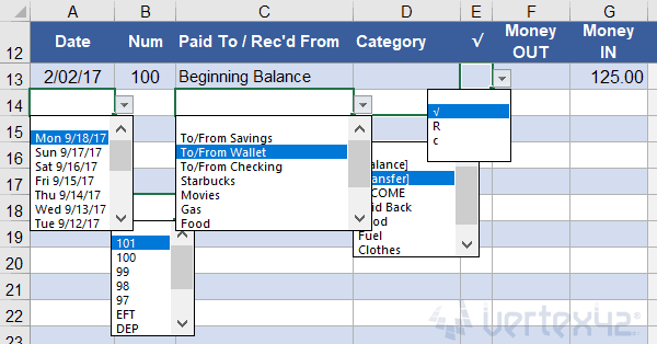 Example drop-down lists in the Money Tracker template for the mobile Excel app.
Jump Ahead To:
- Create a Simple Drop-Down List
- Define a Drop-Down List Using a Range
- Check Boxes and Star Ratings using Drop Down Lists
- Including a Blank Value and Using Relative References
- Copying and Pasting Drop-Down Lists
- Customizable Drop-Down Lists Using Dynamic Ranges
- Dependent Drop-Down Lists Using CHOOSE or INDIRECT
- Fancy Dynamic Drop Downs
- Searchable Drop Down Lists
To see some of the examples from this article in action, download the Excel file below.
Download the Example File (DropDownLists.xlsx)
Watch the Video
Create a Simple Drop-Down List
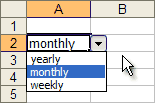 Drop Down List in Excel
You can create an in-cell drop down list in Excel by following these 4 easy steps:
- Select the cell, or range of cells, where you want to add the drop-down list.
- Go to Data > Validation > Settings tab (see image below)
- Select "List" from the Allow: drop-down box
- Enter your list in the Source: field using a comma to separate the items, or select a range of cells from your worksheet.
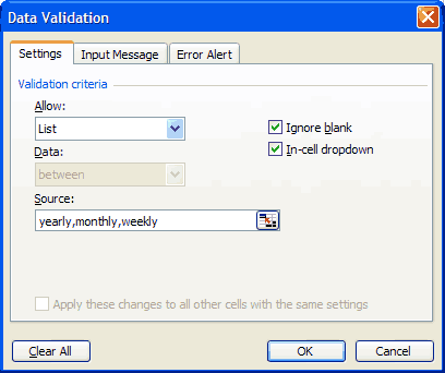 Entering the Source of a Drop Down List as a Comma-Delimited List
This approach is great for simple Yes/No options and other lists that appear only once in your spreadsheet.
The problem with this approach is that if you use this in a lot of cells and later want to update the list, you have to update all cells that use the list and there is a good chance you'll miss one. The more elegant approach is to use a reference to a range, or even better than that - a named range.
Defining a Drop-Down List using a Range
Instead of manually entering the list of items in the data validation dialog box, you can reference a range of cells. For example, let's say I have a separate worksheet with my list defined in cells A1:A3 as shown below. In this case, I've named the range "myList". You can later hide the worksheet containing your list to keep your workbook looking nice and clean or to prevent a user from changing the list.

In the data validation dialog box, instead of entering the list manually, you enter a reference to the named range in the Source field as shown below:
![]()
You could use a reference for the Source field like =Sheet2!$A$1:$A$3, but I usually prefer to name the list. Why? If you want to change the range, you only need to edit the defined name (via Formulas > Name Manager) rather than finding and editing all cells that use that particular data validation.
Note: When using a named range for a data validation list, the named range must be defined as a reference to a range of cells, or it must be a formula like OFFSET or INDIRECT or INDEX that returns a reference. If you're thinking of getting fancy and want to define a name without a cell reference such as ={"Yes","No"}, the drop-down list won't work.
Another bit of trivia: In old versions of Excel, using a named range was the only way for a drop-down list to reference a range on a different worksheet.
Check Boxes and Star Ratings with Excel Drop-Down Lists
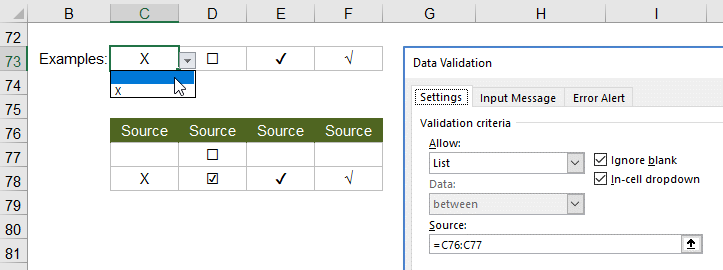
The font used in the drop-down list cannot be changed, so it is always just a black sans serif font. This means that you can't show different colors and fonts within the drop-down list. What I think is awesome, though, is using Unicode Character Symbols to do fun things with drop-down lists, such as star-ratings using ★ or checkboxes using the characters √, ✔, ☐, ☑ or ☒.
Important: One of the main reasons I like to use checkbox-style drop-down lists is for compatibility and ease-of-use with Excel Online and the mobile Excel apps (Form Field checkboxes don't work in Excel Online or mobile apps). Also, when using a touch screen device, I think the drop-down checkbox is easier and more fun to use than entering an "X".
Example 1: Using a Drop Down List to create a Checkbox field
This example comes from one of my Task List templates. The Source field is just "☐,√" (without the quotes).

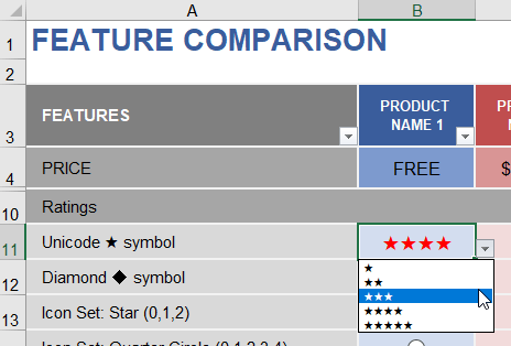
Example 2: Choose a Star Rating using a Drop Down Menu
For a star rating, you can use "★★★★★,★★★★,★★★,★★,★" in the Source field. This example comes from the Feature Comparison template.
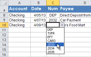
Including a Blank Value and Using Relative References
An in-cell drop down will ignore blanks if you enter text manually into the Source field (like " ,Yes,No"). So, if you want a blank value as an option, use a reference to a range as in the examples below.
Usually, you will use absolute references like $C$76:$C$77 for the Source in your drop-down list. However, there may be times when you want the drop-down Source to change when you copy and paste the cell. In the example above, the drop-downs use a relative reference in the Source field (no $ signs in the reference). This makes it easy to create other checkbox examples by just copying the cells to the right.
Using a relative reference is important when creating dependent lists which will be shown a little later in this article.
Copying and Pasting Drop-Down Lists in Excel
When you copy and paste cells, the data validation will also be pasted, but you can't use the Format Painter to copy and paste data validation. Instead, if you only want to copy and paste the drop-down list (and not formulas or formatting), then after copying the cell, use Paste Special and select the Validation option as shown in the image.

Customizable Drop Down Lists Using Dynamic Ranges
I like creating templates that allow a person to customize lists, such as meals for a Meal Planner or accounts for an Account Register or products for a PO with Price List.
To allow for a variable number of items within the Source range, you could use a very large range like =$A$1:$A$1000, but the drop-down would end up having a crazy amount of blanks. Instead, you can create a dynamic range that extends the list to the last value in the range.
Here is a basic example:

You can see that even though the list range $C$127:$C$133 includes two blank cells, the drop-down only extends to row 131 (the last text value in the Categories column).
Here's how to do it:
Step 1: Create a Dynamic Named Range.
Go to Formulas > Name Manager and create a range named category_list using the following formula in the Refers To field, replacing label_cell and list_range with the appropriate cell references.
=OFFSET(label_cell,1,0,MATCH("zzzzz",list_range,1),1)
Here is the specific formula used in the example.
=OFFSET($C$127,1,0,MATCH("zzzzz",$C$127:$C$133,1)-1,1)
Step 2: Use the Named Range in the Source field for the drop-down list.
Source: =category_list
See my article "Dynamic Named Ranges" to learn more about the various formulas you can use. The formula used in the above example works well for lists that include only text values.
Dependent Drop-Down Lists Using CHOOSE or INDIRECT
A dependent drop-down list is a list that changes based on the value of another cell, which might also contain a drop-down list of its own. The Source for a drop-down list can be a formula, and that is the key to making the dependent list. As I mentioned before, the formula must return a reference, so there are only a few types of formulas that will work for drop downs. I personally prefer using CHOOSE or INDIRECT.
The example below is based on an account register where the idea is to choose categories for each transaction. The Type column contains a drop-down list that references cells C179:D179 (the labels "Expense" and "Income"). We want the dependent drop down box in the Category column to use the list of expenses if the Type is "Expense" and the list of income categories if the Type is "Income."
Here is an example showing the CHOOSE method:
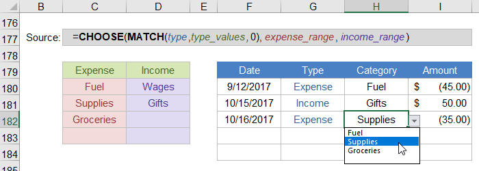
The formula uses a relative reference for the type cell and absolute references for the type_values, expense_range and income_range like this:
=CHOOSE(MATCH(G182,$C$179:$D$179,0),$C$180:$C$183,$D$180:$D$183)
Alternatively, we could create dynamic named ranges called Expense_range and Income_range and then use the following formula for the Source:
=INDIRECT(G182&"_range")
You can use named ranges within the CHOOSE formula as well, so I'm not sure whether one method is better than the other. Some may argue that CHOOSE is better because INDIRECT is a volatile function, but I don't think that matters for drop-down lists.
See the Grocery Price Book template for a practical example of how dependent drop-down lists can be used in a spreadsheet.
Fancy Dynamic Drop-Down Lists
If the previous examples aren't fancy enough for you, my article "Dynamic Drop-Down Lists" explains how to create drop-down lists that change based on user input, the date, check number, etc.
Searchable Drop-Down Lists
If your drop-down list is really long, it can be difficult to find the item you are looking for. Google Sheets provides a great solution, though not a perfect one (yet). In Sheets, you can start typing into the cell and the drop-down list will automatically filter based upon what you type ... as long as it is the start of one or more of the words in the list.
For example, let's say your list contains the names Abe Lincoln, George Washington, Harry Truman, and J. Edgar Hoover. As soon as you type "h", the list will be shortened to Harry Truman and J. Edgar Hoover, but Sheets does not recognize the "h" in Washington.
Excel: Using a fairly complicated trick, you CAN create a searchable drop-down list in Excel. See this youtube video.
More Examples
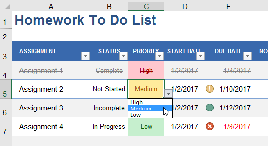
My article Add Cool Features to Your To Do Lists in Excel shows a few other examples, like using conditional formatting combined with a drop-down box to select a priority value in a to do or task list.
Example 1: This Homework To Do List allows you to choose a High, Medium, or Low value in the Priority column. There are also examples of this on the Task List template page.
Example 2: This Task List Template uses conditional formatting icon sets for the Priority column and a drop-down list to choose a value between 1 and 4.
![]()
More Examples: Drop-down lists are a common feature in many of my templates, including the Meal Planner, Money Manager, and many financial calculators. You can download the templates to see how the drop-down lists are created.
The Customer List Template page explains how to copy a customer list worksheet into a spreadsheet, create a drop-down list showing customer names, and then add lookup formulas to display the information for the chosen customer.
Additional Resources
- Create a Drop-Down List at support.office.com - A relatively simple article and video showing how to create a drop-down list in Excel.
- Create and Manage Drop-Down Lists at support.office.com - Includes some very clear videos demonstrating the basics.
The first version of this article was originally published on 4/7/2009 at https://www.vertex42.com/ExcelTips/drop-down-list.html but the original article has been updated and integrated into this blog post.


Comments
Is hiding a list in a separate worksheet the best way (or only way) to stop other users from changing the list?
Most of the time, a drop-down list is used for convenience instead of creating something that is 100% hack-proof. So, if you are just wanting to prevent accidental changes to the list, putting the list on a hidden worksheet is a pretty good solution. That way, if a user really knows what they are doing, they can still change the list (and maybe that’s what you want).
For extra protection, you can password-protect the list worksheet (via Review > Protect Sheet) so that the user cannot change the list even if they figure out a way to unhide the worksheet. For an additional layer of security, you could make the worksheet “very hidden” by going into VBA and changing the Visible property for that sheet to xlSheetVeryHidden, so that the worksheet doesn’t show up in the list of worksheets when a user tries to unhide sheets. However, they could still edit the Source for the Data Validation drop-down list to bypass the original list altogether. Using Review > Protect Sheet will disable the ability to update Data Validation. However, protected sheets are easily hacked, so again – not 100% hack-proof. Unfortunately, Excel does not currently have the option of protecting only specific ranges of cells (unlike Google Sheets).
Thank you for this!
This website has helped me finish a project for my Commander and possible win a company award. Thank you so much and this is an amazing asset!
V/r,
Free D.
Hi there,
Thanks! This is very useful!
Can we generate graphs/charts with spreadsheet that has this drop-down list?
Thanks so much!
@Hani … I don’t see why you can’t. But maybe I’m not understanding your question.
How do I create a drop down list for the gabby chart so I can view the timeline in months?
@Karlee, Assuming you mean Gantt chart, creating a drop-down list isn’t the hard part. The hard part is updating all of the other formulas and labels to make it work for displaying and calculating differently based on what you select in the drop-down. The Pro version already has that functionality built in.
i am trying to create a drop down pick list I have the data on sheet 1, column A has the description, and column B has the cost.
What I want to acheive in the other Sheets is a “Order Sheet” They would be able to use the drop down list (which I can acheive from the above help using the data validation) But what I can’t figure out is how to carry over the cost in column B on full list. So the User can use Sheet 2, “Order Sheet” select the part they want on each line (that I have as a drop down) then column B should also get carried over and the Order Sheet could SUM up the total of items selected, to insure the stay under the specific budget. This was they can mix and match parts wanted to see different totals populate – if that makes sense.
@Dan, To select the Cost for a given Order (assuming the Order is a unique value in the original table), I think you may find what you are looking for in the VLOOKUP and INDEX-MATCH article.
Hi! Love your purchase order templates!! How do I re-write the formula so the price list drop down searches for item # instead of description?
@Mary … First, create a drop-down list for the Item # column using the method described in this article. Then you can use an INDEX-MATCH formula in the description column to return the description by looking up the item #. If you need help with that, read the article about lookup formulas and analyze the formula in the ITEM # column of the purchase-order_pricelist.xlsx file.
Hi! I’m new at Excel and I am having issues trying to get my searchable drop down list to search quicker. I have the drop down list working but it is extremely slow at generating the numbers visible from the drop down box. Is there any way I can speed it up?
@Sam, You might need to have a consultant take a look at your file. There is a very detailed article about how to create a searchable drop down list here. You might consider posing your question on that blog article, assuming you have created your searchable drop down list using the same technique.
Hai Sir Can u sent a video money tracker excel sheet making
I’m not sure what you are asking, exactly. I don’t have a video showing how to make the Money Tracker spreadsheet, but there is a video demo about it, and the video at the top of this page shows how to create a dropdown in Excel. I do think it would be a good idea to create a video to demo the Money Tracker, so I’ll that to my to do list.
Hi,
I am creating a client database. I have multiple headings such as, name, contact info, email etc etc. I have more than 1 person for each company. I want to compile all of this data into one tab which I can get from the drop down list, is this possible?
Thanks
Ashlee
It should be. You’ll want a column for “Company” also. See the Customer List Template or the CRM Template,
I am going to use your Food Diary for monitoring interaction of food with Dr. prescribed physical therapist exercises to address very elderly sarcopenia.
I would like to add some columns to the FoodList (Fiber, Sodium, Potassium, Calcium) and have then carry over to the FoodDiary.
I was able to add the columns to the FoodList OK, but don’t know how to add the columns to the FoodDiary so that I can complete the process.
Could you explain how to do that for a person with limited in Excel skills?
Is it possible to have two FoodDiary tabs with the one FoodList so that husband and wife could use same spreadsheet for different diets?
Thank you very much for all that you do to help others with practical Excel spreadsheets.
John
You’ll need to look at the existing formulas in the FoodDiary worksheet and figure out how to make them work for new columns that you add. After you insert more columns into the table in the FoodList worksheet, the VLOOKUP functions may become messed up because they refer to specific columns by number. So you’d need to update those numbers. Get the formulas in the first row to work, then you can copy them down. For help with customization, you could contact ExcelRescue.net for a quote.
Hi. I’ve looked and I don’t see anything on your site that records price history. For example, I’d like to record the price I pay for specific items on a particular date. Then I could have it calculate the lowest, highest, and average price paid for that item. That would be very handy to be able to look at an item’s current price and compare how the price compares to what they’ve sold it for in the past to decide if I want to purchase it now, wait for the price to come down, or search for the item elsewhere. Plus, it would be a great way to assist other family members who are helping make household purchases so as not to pay too much for items. Thanks!
The Price List template could probably be modified fairly easily to include a Date column. Thanks for the suggestion!
I want to hide the cells instead of giving grey color, how to hide cells for unselected customers data
You mean hiding rows? or just making a cell appear to be blank? You can use conditional formatting to make a cell value appear to be blank by using a custom number format of “;;;”.