
VLOOKUP and INDEX-MATCH formulas are among the most powerful functions in Excel. Lookup formulas come in handy whenever you want to have Excel automatically return the price, product ID, address, or some other associated value from a table based on some lookup value. The VLOOKUP function can be used when the lookup value is in the left column of your table or when you want to return the last value in a column. The INDEX and MATCH functions can be used in combination to do the same thing, but provide greater flexibility without some of the limitations of VLOOKUP. I'll also mention LOOKUP and CHOOSE and EXACT and ISBLANK and ISNUMBER and ISTEXT and ... 🙂, but this article is mainly about VLOOKUP and INDEX-MATCH.
To see these examples in action, download the Excel file below.
Download the Example File (LookupFormulas.xlsx)
Do you have a VLOOKUP or INDEX-MATCH challenge you need to solve? If you can't figure it out after reading this article, go ahead and ask your question by commenting below.
This Article (bookmarks):
- Simple VLOOKUP and INDEX-MATCH Examples
- Wildcard Characters for Partial Match Lookups
- Approximate Match Lookups (for Grades, Discounts, Taxes, etc.)
- 2D Lookups Using VLOOKUP-MATCH and INDEX-MATCH-MATCH
- 3D Lookups Using INDEX-MATCH and VLOOKUP
- Case-Sensitive EXACT Lookup Using INDEX-MATCH
- Multiple-Criteria Exact Lookups Using VLOOKUP and INDEX-MATCH
- Lookups with Multiple Non-Exact Criteria Using INDEX-MATCH
- Return the Last Numeric Value in a Column
- Return the Last Text Value in a Column
- Return the Last Non-BLANK Value in a Range
- Return the Last Non-Empty Value in a Range
- Lookup based on the Nth Match
1) Simple VLOOKUP and INDEX-MATCH Examples
VLOOKUP Example
First, here is an example of the VLOOKUP function using a simple Price List Table. We're looking for the text "a_003" within the Item ID column and wanting to return the corresponding value from the Price column.
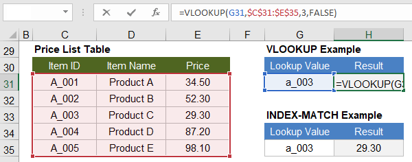
=VLOOKUP(lookup_value,table_array,col_index_num,FALSE)
How it works: The table_array argument is a range that must have the lookup column on the left. The price column is the 3rd column in the highlighted range, so that is why the col_index_num argument is 3 in our example. We use FALSE for the final argument because we want the VLOOKUP function to do an exact match.
NOTES Actually, this lookup is not truly "exact" because both VLOOKUP and MATCH are not case-sensitive, but the syntax tooltip in Excel calls the option an "exact match" so we'll just accept that and explain how to do a case-sensitive match later.
If you later insert a column in the middle of your table_array, the Price column might not be column 3 any more. To prevent your VLOOKUP formula from breaking, in place of the 3 in the example, you can use (COLUMN($E$30)-COLUMN($C$30)+1).
The default for VLOOKUP is not an exact match, so don't forget to include FALSE as the 4th argument if you want an exact match.
INDEX-MATCH Example
Next, you'll see that the INDEX-MATCH formula is just as simple:
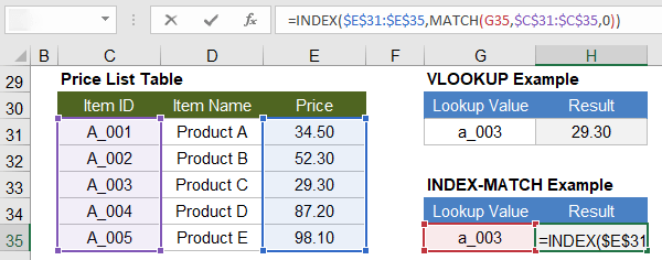
=INDEX(result_range,MATCH(lookup_value,lookup_range,0))
How it works: The MATCH function returns the position number 3 because "a_003" matches the 3rd row in the Item ID range. Next, INDEX(result_range,3) returns the 3rd value in the price list range.
The INDEX-MATCH formula is an example of a simple nested function where we use the result from the MATCH function as one of the arguments for the INDEX function. The example below shows this being done in two separate steps.
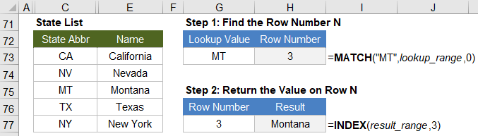
Syntax and Notes for MATCH and INDEX
MATCH returns the position number of a matched value within the lookup range.
=MATCH(lookup_value,lookup_range,match_type)
NOTES When using MATCH, the lookup_range can be a row or column, but if lookup_range is more than one row or column, MATCH will return an error.
MATCH returns the #N/A error when it does not find a match.
The match_type is optional, but the default is not 0. So, it is is best to always specify the match type.
INDEX returns a value from an array based on a row and column number.
=INDEX(array,row_number,[column_number],[area_number])
NOTES You don't need to include the optional column_number if the array is a single column.
The optional area_number argument is only used for 3D arrays.
If your array is a row, don't use the shortcut =INDEX(array,column_number) because that may not be compatible with other spreadsheet software. Use =INDEX(array,1,column_number) instead.
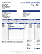 Purchase Order with Price List
See INDEX-MATCH in action. In this template, you choose an Item Description from a drop-down list, then lookup formulas display the Item # and the Unit Price for that item.
2) Use Wildcard Characters (?, *) for Partial Matches with VLOOKUP and INDEX-MATCH
Wildcard characters can be used within the lookup_value for both VLOOKUP and MATCH formulas when the lookup is text and you are doing an exact match.
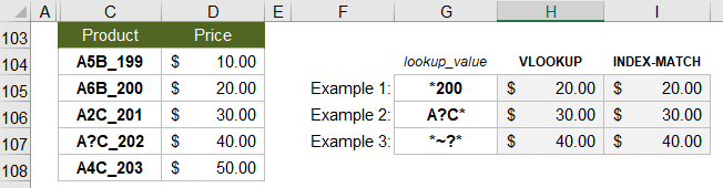
* (asterisk) matches any number of characters. For example, use "*200" to find the first value ending in 200.
? (question mark) matches any single character. For example, use "A?C*" to find the first value where "A" is the first character and "C" is the 3rd character. The second character can be anything, but only a single character.
~ (tilde) is used in front of a wildcard character to treat it as a literal character. In the 3rd example, we use "*~?*" to find the first occurrence of a product that contains an actual question mark.
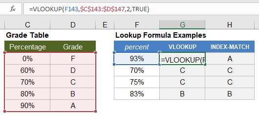
3) Return Approximate Matches Using VLOOKUP and INDEX-MATCH
The following examples show how to use VLOOKUP and INDEX-MATCH to return approximate matches with numerical lookup data. Important: When using an "Approximate Match" with VLOOKUP (where the 4th argument = TRUE) and a "Less than" match with MATCH (where the 3rd argument = 1), the lookup range needs to be sorted in ascending order.
These formulas look for the largest value that is less than or equal to the lookup value.
=VLOOKUP(lookup_value,table_array,col_index_num,TRUE)
=INDEX(result_range,MATCH(lookup_value,lookup_range,1))
Example 1: Return a Grade based on Percent
► See this in action: Download the Grade book Template
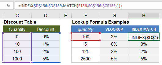
Example 2: Return a Discount Rate based on Quantity
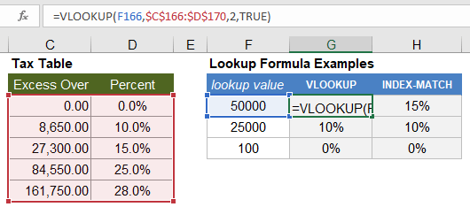
Example 3: Return a Tax Rate based on Income
► See this in action: Download the Paycheck Calculator
CAUTION For an approximate match, these formulas use a very efficient search algorithm that assumes the lookup range is sorted in ascending order. If your data is not sorted, they don't return an error value, but the result may be unpredictable.
If the lookup value is less than the first value in the lookup range, MATCH and VLOOKUP will return an error.
4) 2D Lookups Using VLOOKUP-MATCH and INDEX-MATCH-MATCH
In this example, we'll do a mileage lookup between two cities. The formulas are basically the same as for a 1D lookup, except that we use a MATCH function to replace col_index_num in the VLOOKUP function and to replace column_number in the INDEX function.
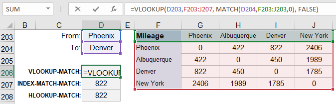
Using VLOOKUP
=VLOOKUP(row_lookup_value,table_array, MATCH(column_lookup_value,column_label_range,0), FALSE)
Using INDEX-MATCH-MATCH
=INDEX( result_array,
MATCH(row_lookup_value,row_label_range,0),
MATCH(column_lookup_value,column_label_range,0) )
Using HLOOKUP
=HLOOKUP(column_lookup_value,table_array, MATCH(row_lookup_value,row_label_range,0), FALSE)
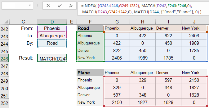
5) 3D Lookups Using INDEX-MATCH and VLOOKUP
To demonstrate a 3D lookup, we'll use mileage tables again, but this time we have a separate table for Road and Plane. The INDEX function allows you to return a value from a 3D array. You can replace the row_number, column_number, and area_number with 3 MATCH functions.
NOTE The reference argument for the INDEX function should be multiple same-size ranges surrounded by parentheses like this: (A1:D10,E1:H10), or you can use a named range.
=INDEX( (array_range1,array_range2) ,
MATCH(row_lookup_value,row_label_range,0),
MATCH(column_lookup_value,column_label_range,0),
MATCH(table_lookup_value,{"Road","Plane"},0) )
3D Lookup Using VLOOKUP
It is possible to do a 3D lookup using VLOOKUP. Starting with the 2D lookup formula, in place of array_table, you can use CHOOSE(table_number,table_array_1,table_array_2). You can use MATCH to find the value for table_number as in the INDEX-MATCH example above. The resulting formula would look like this:
=VLOOKUP(row_lookup_value, CHOOSE( MATCH(table_name,{"Road","Plane"},0), road_table_array, plane_table_array), MATCH(column_lookup_value,column_label_range,0), FALSE)
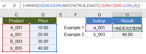
6) Case-Sensitive EXACT Lookup Using INDEX-MATCH
Most lookups and logical comparisons in Excel are NOT case-sensitive, meaning that both "A"="a" and "A"="A" would return TRUE.
The EXACT(value1,value2) function allows you to make a comparison between value1 and value2 that IS case sensitive, so EXACT("A","a") returns FALSE and EXACT("B","B") returns TRUE.
If you use EXACT to compare a value to a range like EXACT("B",A1:A20), the function returns an array of TRUE and FALSE values. You can then use a MATCH function to look for the value TRUE within the range returned by EXACT(lookup_value,lookup_range). The final lookup formula is an Excel Array Formula, so you need to press Ctrl+Shift+Enter after entering the formula.
{Ctrl+Shift+Enter} =INDEX(result_range, MATCH(TRUE,EXACT(lookup_value,lookup_range),0) )
See the references at the end of this article if you are curious about how a case-sensitive lookup can be done with VLOOKUP.
7) Multiple-Criteria Exact Lookups Using VLOOKUP and INDEX-MATCH
One way to do an exact-match using multiple criteria is to concatenate the lookup columns and do a lookup using the concatenated lookup values. VLOOKUP requires using a helper column containing the concatenated lookup columns. INDEX-MATCH does not need the helper column, but it becomes an array formula (Ctrl+Shift+Enter).
Multiple-criteria lookup using VLOOKUP and a helper column
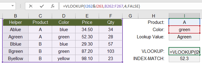
=VLOOKUP(value_1 & value_2,table_array,col_index_num,FALSE)
Multiple-criteria lookup using INDEX-MATCH as an array formula
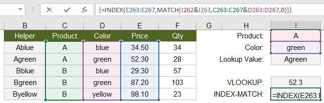
{Ctrl+Shift+Enter} =INDEX(result_range,MATCH(value1 & value2, lookup_col1 & lookup_col2,0))
8) Lookups with Multiple Non-Exact Criteria Using INDEX-MATCH
When you want to use logical conditions such as A > B or A < B in your lookup, a method I like is to use INDEX-MATCH and convert the lookup_range to a TRUE or FALSE expression like lookup_range<lookup_value. Then search for the first occurrence of TRUE (using 1 as the first argument of the MATCH function). Using this method, you can have any number of conditions because multiplying true/false expressions together acts like the logical AND operator. The formula must be entered as an array formula (Ctrl+Shift+Enter), but that's a small price to pay for relative simplicity.
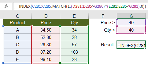
{Ctrl+Shift+Enter} =INDEX(result_range,MATCH(1, (lookup_col1>lookup_value1) * (lookup_col2<lookup_value2) ,0) )
9) Return the Last Numeric Value in a Column
When using an approximate lookup for VLOOKUP and MATCH, you can return the last numeric value in a column if you use an extremely large number as the lookup value (to make sure it will be larger than any number in the lookup range). A common example would be to return the last value in a Balance column for a checkbook register as shown in the example below.
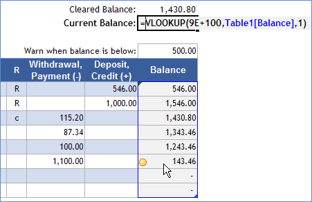
=VLOOKUP( 9E+100, lookup_column, 1, TRUE)
Recall that the TRUE option (for an approximate match) is the default for VLOOKUP, so that is why the formula in the checkbook example image only shows 3 arguments.
This can of course be done with INDEX-MATCH, but I prefer the VLOOKUP formula in this case because it requires only one reference to the lookup column.
=INDEX( lookup_column, MATCH( 9E+99, lookup_column, 1) )
NOTES The lookup_column can contain text values and even errors (like #N/A or #DIV/0), and those values will be ignored. The formula returns only the last numeric value.
10) Return the Last Text Value in a Column
When searching for the last text value, instead of a large numeric value for the lookup_value as in the previous example, use a "large" text value. By that, I mean a text value that would show up last if you sorted a column in alphabetical order. If you are using the English alphabet without special characters, that could be "zzzzzz." If you are using Greek characters or symbols in your list, you could try a Unicode Character such as "🗿" as the lookup value.
=VLOOKUP( "zzzzzzz", lookup_column, 1, TRUE)
=INDEX( lookup_column, MATCH( "🗿", lookup_column, 1) )
Rather than returning the last text value, I often use just the MATCH part of this formula to return the row number of the last value. This allows you to make a dynamic named range that can be used as the source range for a drop-down list via data validation.
11) Return the Last Non-BLANK Value in a Column
If your column contains both text and numeric values, you may want a formula to return the last non-BLANK value. Using the INDEX-MATCH formula, we can search for the last numeric value and the last text value and return whichever comes last.
=INDEX( lookup_column, MAX( MATCH( "zzzzzz", lookup_column, 1), MATCH(9E+100, lookup_column,1) ) )
A more concise formula uses the LOOKUP function. The LOOKUP function allows the lookup_range to be an expression rather than a direct reference (and it can be a row or column). We can use a logical comparison and search for the last TRUE value like this:
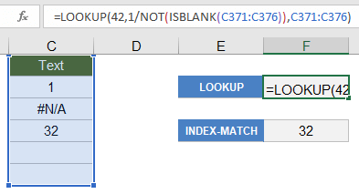
=LOOKUP(42, 1/NOT(ISBLANK(lookup_range)), lookup_range)
The trick here is that the expression 1/NOT(ISBLANK(lookup_range)) returns an array of 1s for TRUE and #DIV/0 errors for FALSE. LOOKUP ignores the error values so it will return the last value in lookup_range that is not blank. The number 42 is arbitrary - it just needs to be larger than 1 to return the last value.
Using very similar formulas, you can use LOOKUP to return just the last numeric value or text value like this:
=LOOKUP( 42, 1/ISNUMBER(lookup_range), result_range)
=LOOKUP( 42, 1/ISTEXT(lookup_range), result_range)
12) Return the Last Non-Empty Value Using LOOKUP
If you are using a formula to return an empty value "" and you want to ignore those cells when searching for the last value in the range, you can use the LOOKUP formula mentioned in the last example with the expression 1/(lookup_range<>"").
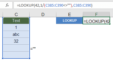
=LOOKUP(42, 1/(lookup_range<>""), lookup_range)
If you want to return the relative row number instead of the actual value, you can use the following formula:
=LOOKUP(42, 1/(lookup_range<>""), ROW(lookup_range)-ROW(first_cell_in_lookup_range)+1 )
13) Lookup based on the Nth Match
You can use the SMALL function to return the Nth smallest value from an array, and we can use that along with an array formula and the INDEX function to do a lookup based on the Nth match. See my Array Formula Examples article to learn more about Array Formulas and specifically the SMALL-IF formula.
In this example, we want to return the 2nd Event that matches the date 3/7/2018. Note: The curly { } brackets in the formula below are a reminder to press Ctrl+Shift+Enter to enter the formula as an Array Formula. You don't actually type the brackets into the formula.
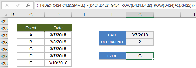
{ =INDEX(result_range,SMALL( IF(lookup_range=lookup_value, ROW(lookup_range)-ROW(first_cell_in_lookup_range)+1),occurrence)) }
How does this work? The SMALL-IF part of the formula is acting kind of like the MATCH function except that it is returning the index number for the 2nd occurrence of the match. We can use SMALL in this example because Excel stores dates as numbers.
This formula is used within the Daily Planner Template to list events and holidays occurring on a particular date.
14) VLOOKUP vs. INDEX-MATCH
Excel people like to debate about whether VLOOKUP is better than INDEX-MATCH for lookup formulas. The most common argument is that VLOOKUP is simpler and INDEX-MATCH is more powerful. Even though I usually prefer INDEX-MATCH, I think both formulas are pretty simple, and one isn't necessarily always more powerful than the other.
If you want to do more advanced lookups with VLOOKUP, then you'll probably need to learn how to use MATCH and CHOOSE. If you want to become a power Excel user, then you'll also want to learn the INDEX function. So, my opinion on the VLOOKUP vs. INDEX-MATCH debate is to learn how to use them all.
In conclusion, here are some reminders applicable to both VLOOKUP and INDEX-MATCH:
- Don't forget the FALSE or 0 option if you are wanting an exact match, because the default parameter is to use an approximate match.
- As a general rule, use absolute ($A$1) cell references to refer to the lookup ranges and table arrays because when you copy the lookup formula you will usually want those ranges to remain the same.
- Check for extra blank spaces if you think a lookup formula should be finding a match, but it is not.
- Use IFERROR to handle the error returned when an exact match is not found.
References
- Spreadsheet Tips Workbook - vertex42.com - by Jon Wittwer and Brent Weight
- VLOOKUP Function - support.office.com - The official documentation of the VLOOKUP function.
- MATCH Function - support.office.com - The official documentation of the MATCH function.
- INDEX Function - support.office.com - The official documentation of the INDEX function.
- Case-Sensitive Match Using VLOOKUP - at ablebits.com - This shows that it IS possible, but the solution is quite complex.
- Get Value of Last Non-Empty Cell - at exceljet.net - I think this article explains the LOOKUP function better than I did.


Comments
I’ve seen MATCH(“*”,range,-1) used to find the last text value. Isn’t that a bit better than using “zzz” or some special character?
@Jeremy, Using MATCH(“*”,range,-1) is not a very robust formula for finding the last text value. Text beginning with some characters like !, $, (, or even a leading space will cause the formula to not necessarily find the last text value. That is because when using the -1 value for the 3rd argument (instead of 0 for exact match), an asterisk is not a wildcard – it is treated as the literal * character.
I want to do a lookup based on the 2nd occurrence of some value in a list. I know that SMALL or LARGE can return the 2nd occurrence of a value, but I need to do a lookup that returns a value from a different column, not the same column. Is that possible?
@Jeff, You can use an array formula to do a lookup based on the nth match. I will add this example to the blog post.
Wonderful examples and spreadsheets with examples, thank you!
I AM TRYING TO INDEX A LARGE RANGE WITH SEVERAL CRITERIA THAT HAVE TO MATCH. I CAN’T SEEM TO GET THE FORMULA TO WORK SO THAT IT WILL FIND THE CORRECT COLUMN TO GIVE THE RESULT
{=INDEX((Register!J5:BC42),MATCH(Register!$C$11:$C$42=’Weekly Reports by Dept.’!DB$1, 0),MATCH(Register!$D$11:$D$42=’Weekly Reports by Dept.’!DA$1, 0),MATCH(Register!J5:BA5=”REGHRS”, 0))}
@Helen, Your formula looks like a 3D lookup rather than a multi-criteria lookup (or maybe a 2D lookup combined with multiple criteria for the row?). A 3D lookup might be considered a multi-criteria lookup, but a multi-criteria lookup is not necessary 3D. 3D has to do with how your data is structured (e.g. lookup value in a row and column within multiple ranges). To do a multi-criteria lookup such as A1 AND A=2 AND B=3 usually involves concatenating the criteria and matching the concatenated result. For consulting help on a specific problem, I’d recommend ExcelRescue.
I have an database whereby I wish to replace partial text in a string using a vlookup in a table on a separate worksheet as follows:
Worksheet1:
A1: this is a test replacement for MPv3 filename
A2: filex32 exists
Worksheet2:
Table Replacement
Mpv3 MP3
MPv4 MP4
b@listic balistic
/
x32 x86
Ideally a substitute function in Column B fields 1 & 2 would show as per below:
A1: this is a test replacement for MPv3 filename
A2: filex32 exists
B1: this is a test replacement for MP3 filename
B2: filex86 exists
I assume the calculation to substitute the text in A1 would use a vlookup and substitute function.
Thanks in advance for your assistance.
Regards,
David
@David, Yes I think you are right. Something like INDEX(Sheet2!B:B,MATCH(“MPv3”,Sheet2!A:A,0)) to look up the replacement for “MPv3”. So B1 might be =SUBSTITUTE(A1, “MPv3”, INDEX(Sheet2!B:B,MATCH(“MPv3”,Sheet2!A:A,0)) )
I have an excel file in which I need to compare two columns for duplicate data, and the third column should reproduce the duplicated entries. Can that be made possible with index match formula?
@Aayushi, Yes. INDEX-MATCH could be used to check whether the value in cell A1 matches a value in column B, then that formula could be copied down. For example: C1=INDEX(B:B,MATCH(A1,B:B,0)).
I have an excel file in which I need to compare two columns for BIN_NO and CODE and get the corresponding BATCH and COST
BIN_NO CODE Batch Cost
12061 1 1540 $120,611 BIN_No 12061
12061 2 1663 $120,612 CODE 3
12061 3 1812 $120,613 Batch
12061 4 1712 $120,614 Cost
12071 1 1681 $120,711
12071 2 1738 $120,712
12071 3 1540 $120,713
12071 4 1370 $120,714
12081 1 2704 $120,811
12081 2 1540 $120,812
12081 3 1812 $120,813
12081 4 1712 $120,814
@DJ – That sounds like a multi-criteria lookup. See section 7 in the article.
I have a question on the array formula using nthmatch let me know if sending example via email will help
@Keyri, Go ahead and send an email. Or, you could contact ExcelRescue.net if it is something complicated that you need help customizing.
I think that your G31 and G35 the LOOK_UP VALUE in your first two examples should be C33.
@Jerry … no, the lookup value in the formula is G31. The formula is used to find the row containing the value in cell G31 (you could replace G31 with “a_003”) and then return the associated price from the 3rd column of the lookup range.
Hi, Could you please let me know what formula I should use for the following file? For example, I have 5 suppliers offered different prices for different items. I have decided to select the final supplier according to the cost and material. I have highlighted the selected prices in Green color. How can I get the Final cost by using auto-search formula? Because I have thousand items, it’s very time consuming to select one by one. Thank you very much for your help!
Supplier1 Supplier2 Supplier3 Supplier4 Supplier5 Final cost
Item 1 0.2 0.5 0.46 0.3 0.33 0.33
Item 2 2 2.6 3 2.3 2.7 2.3
Item 3 5 4.2 4.5 4.3 4.8 4.2
Item 4 6.3 5.4 5.8 6 5.5 5.8
Item 5 3.5 4 4.2 3.8 4.5 4
This is great article. The problem with Vlookup is that so many different uses of it. I found out, its never enough to know how many ways there are to use Vlookup.
hi great website
do u have a template of vlookup that has the ablity to read the sum cell?like in fol a
there are then jacks
cupboard diffrentscore
Hey Guys
I am sure there is something that can help me above but I am a little pushed for time so I am hoping that if I describe my spreadsheet and what I want it to do you can point me to the right solution and then I can study it to formulate, or even better give me the steps ;) .
I have a workbook that I paste restaurants sales/banking/cashup data into my date tabs, 1st, 2nd, 3rd, etc. I built a pretty good summary page to bring each days data into the one sheet based on a vlookup to the dropdown restaurant name, 1st row selects from 1st tab, 2nd row selects from 2nd tab, etc.; however, this is all based on column numbers, so if any of these columns change for some reason, extra columns added in the POS report format, my workbook is going to go out of whack. So, I am thinking I need to do Index/Match somehow but I also need it to Vlookup the restaurant name, so I need it to look up the restaurant name which I have in a dropdown box in A1, I have the dates of the given month listed vertically in column B, this can be shifted to column A if need be, then the names of the columns consist of gross sales, cash takings, card, account, tips, etc., I need to pull the data from each of my 31 tabs (days of the month), so lookup restaurant name and pull the gross sales for the 1st December by looking in the 1st tab, in each of the tabs, all the restaurants are listed in column A vertically, the gross sales, cash, card, etc., listed horizontally.
I hope this makes sense, if you could point me in the right direction, help me out, that would be so helpful. Thank you
Normally, I’d point you to this blog post for help with Vlookup and Index-Match. But if that doesn’t help, you could contact ExcelRescue.net to get a quote for Excel help.
I am trying to look up a value with two references. Is that possible?
HI,
I have the following Spreadsheet.
A1:A1000 = Dates (in date order)
B1:B1000 = Values (in date order)
C1 = Date I want to look up
D1 = Value I want to look up
F1= //Answer
I want to look for C1 in Column A and then from that row look down for a value <= D1 and then return the Date in Column A to F1.
Is that possible?
Thanks in advance
Not using the regular lookup functions. You could probably do something like this with an advanced array formula. You could first use a lookup to return the row matching C1, and use the OFFSET function to create a new range for performing the second stage lookup.