Dynamic Arrays in Excel are fundamentally important to understand if you are going to do any data manipulation, matrix math, or create formulas having to do with ranges and arrays. If all you do is read the "Need to Know" section, that may be sufficient for now, but this article also reviews the new Excel array functions.
Download the accompanying Excel file to see the examples in this article in action:
Download the Example File (DynamicArrays.xlsx)
Table of Contents
Dynamic Arrays : Need to Know
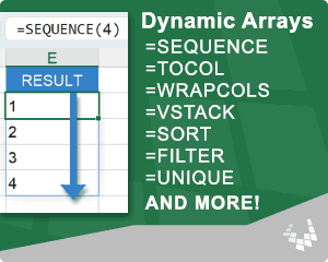
#1: The SEQUENCE Function
The SEQUENCE function may be the most commonly used dynamic array function. For example, to create a sequence of numbers from 1 to 50, enter =SEQUENCE(50). See below for more examples.
#2: The "Spill" Behavior
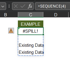
A "Dynamic Array" is also called a "Spilled Array" because of the "Spill" behavior: When a formula would return more than one result, the results automatically spill into the next rows or columns. If the result would overrun existing data in your spreadsheet, you will see the #SPILL! error instead.
Solution to #SPILL!: Either reduce the size of your returned array, move your formula to where you have more room, or move your existing data.
#3: The # Character
You reference the result of a dynamic array using the # character after the first cell in the array. For example: instead of =$C5:$D100, it's just =$C5#. This is how you can reference the entire dynamic array instead of manually adjusting the reference any time the array size changes.
#4: Link a Chart to a Dynamic Array
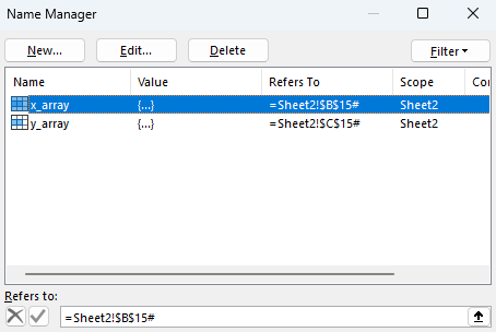
If you want to link a series in a chart to a dynamic array, you can't use the # notation directly in the series range fields. Instead, you first name the array using the Name Box or the Name Manager, then use that named range to define the chart series. Here's how:
First, create names for the arrays using the # notation in the Refers to field. (I prefer using worksheet scope rather than workbook scope, but it will work either way). The image below shows these arrays named x_array and y_array.
Second, set up the chart like normal and then select the data series in the chart. In the formula bar, change the $C$15:$C$29 part of the reference to the named range (y_array in this example). You still need the worksheet reference, so in this example you wouldn't delete the Sheet2! part of the reference.
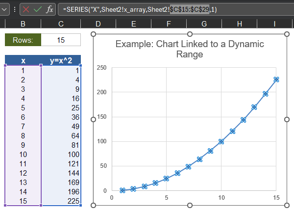
Download the example file above and go to Sheet2 to see this example in action. You can change the number of rows and the chart updates automatically.
#5: Upgrade
If you can't do any of these new cool things because you are using an old version of Excel, it's time to upgrade Excel to a Microsoft 365 subscription. And for even more cool things, join the Insider program (just a few clicks: File > Account > Microsoft 365 Insider, then a restart).
We're done! Those are the most important points, so you can move on to LAMBDAs, or continue reading for an overview of more dynamic array functions.
Or, instead of reading the article, download the following Excel file and scroll through the examples:
Download the Example File (DynamicArrays.xlsx)
Other Details about Dynamic Arrays
The Microsoft Support article about dynamic arrays provides a decent overview, so if you have already read that, you can skip down to the examples.
Blue Border : When you select a cell within the dynamic array, you'll see a blue border marking the current boundary of the array.
Navigate to the Start Cell : Ctrl+a then Ctrl+Alt+Arrow. When working with large arrays, it may be useful to quickly navigate to the first cell in the dynamic array. Use this shortcut while you have at least one cell in the array selected.
@ Character : If you intentionally want your dynamic array formula to return only the first result, then you can precede the function with the @ symbol.
ROWS(C36#) : Returns the number of rows within the dynamic array C36#.
COLUMNS(C36#) : Returns the number of columns within the dynamic array C36#.
Old "Legacy" Ctrl+Shift+Enter array formulas: most of the old array formulas still work in the newer versions of Excel, but you don't usually need to use Ctrl+Shift+Enter any more (though they can sometimes behave differently if you do not, so test them).
The SEQUENCE Function
=SEQUENCE(rows,[columns],[start],[step])
SEQUENCE is my favorite dynamic array function - I definitely use it the most. Here are few examples to create various sequences.
The LET Function : While not specifically what this article about, you'll see that I'm using the LET function in the following examples. This isn't necessary, but I like doing this because (1) it helps you see what variables are used for each formula and (2) you can copy and paste the example formula directly into Excel.
Create a Sequence of Dates
=LET(
    start_date, DATE(2024,1,1),
    step, 7,
    cols, 5,
    SEQUENCE(1,cols,start_date,step)
)

Result: {1/1/2024, 1/8/2024, 1/15/2024, 1/22/2024, 1/29/2024}
Actually, the result will be the date serial numbers until you format the cells as dates.
Create a Sequence of N values from Start to End
This example may be my favorite way of creating series for charts. This formula works like the linspace function in MATLAB.
=LET(
    start, 2,
    end, 10,
    n, 5,
    SEQUENCE(1,n,start,(end-start)/(n-1))
)

Result: {2, 4, 6, 8, 10}
Create a Sequence of Integers from Start to End (For j = 5 To 1)
When you want a sequence of integers that may start at a value other than 1 and might involve a negative step, this function comes in handy.
=LET(
    start, 5,
    end, 1,
    SEQUENCE(1,start-end+1,start,IF(end<start,-1,1))
)

Result: {5, 4, 3, 2, 1}
Create a Sequence of Month Names
=TEXT(EDATE(DATE(2020,1,1), SEQUENCE(1,12,0)), "mmm")

Result: {"Jan","Feb","Mar","Apr","May","Jun","Jul","Aug","Sep","Oct","Nov","Dec"}
This function depends on language settings because of the TEXT formula and the "mmm" format code.
Create a Sequence of Characters
=LET(
    start, "A",
    n, 5,
    UNICHAR(SEQUENCE(1,n,UNICODE(start)))
)

Result: {"A","B","C","D","E"}
The TOCOL and TOROW Functions
=TOCOL(array,[ignore],[scan_by_column])
=TOROW(array,[ignore],[scan_by_column])
TOCOL converts an array into a single column of values (stacking the values on top of each other). TOROW converts the array into a single row of values. The default scan direction is by row, meaning scanning from left to right one row at a time. The scan_by_column argument can be set to TRUE to scan down each column.
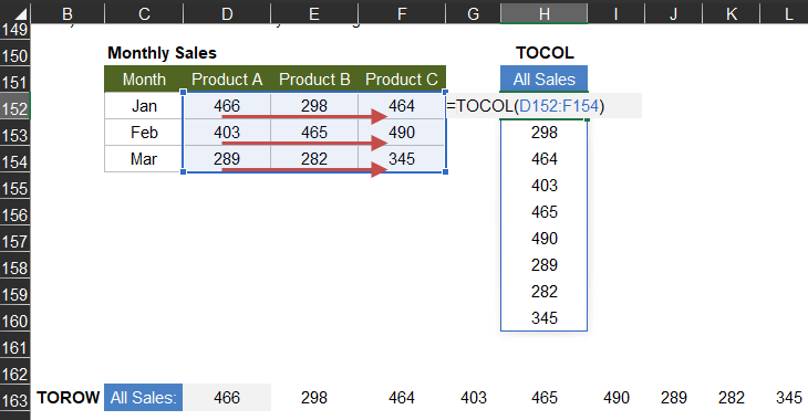
TIP =TOCOL(range,3) is a quick way of removing blanks and errors from a column of data (vs. FILTER).
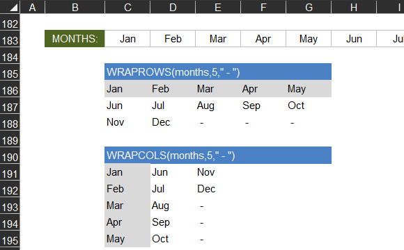
The WRAPCOLS and WRAPROWS Functions
=WRAPCOLS(vector, wrap_count, [pad_with])
=WRAPROWS(vector, wrap_count, [pad_with])
WRAPCOLS and WRAPROWS are essentially the opposite of TOCOL and TOROW. They allow you to take a single column or row of values and wrap them into an array of a particular number of rows or columns.
WRAPROWS wraps the values of the original array into rows, starting with row 1, then row 2, then row 3, so you need to define the number of columns in each row, or the column number after which the rows will be wrapped. It doesn't matter whether the original array is 1xn or nx1.
WRAPCOLS wraps the values of the original array into columns, starting with column 1, then column 2, etc. so you need to define the number of rows.
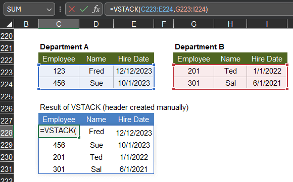
The VSTACK and HSTACK Functions
=VSTACK(array1,[array2],[array3],...)
=HSTACK(array1,[array2],[array3],...)
These functions come in very handy when you are manipulating and assembling arrays by putting pieces together. VSTACK will combine arrays by stacking them on top of each other. This may be useful for combining data from multiple worksheets and tables. HSTACK is similar, but stacks horizontally rather than vertically. The arrays can be of different sizes, but the blanks will be filled with NA().
ARRAYTOTEXT
=ARRAYTOTEXT(array,[format])
I'm not sure this really is a dynamic array formula because the output is just one result, but I'll include it here anyway. ARRAYTOTEXT converts an array to a string of values separated by commas. The [format] option is either 0 for comma separated values, or 1 for a string that includes curly braces and quotes around strings. This second option (format=1) is important because the result is an official array string that you can use within Excel formulas.
format=0 is basically the same as using TEXTJOIN(", ",,array).
Here is a sequence of weekday names, converted to an array string:
=TEXT(SEQUENCE(1,7,DATE(2024,1,1)),"ddd"))

Result: {"Mon","Tue","Wed","Thu","Fri","Sat","Sun"}
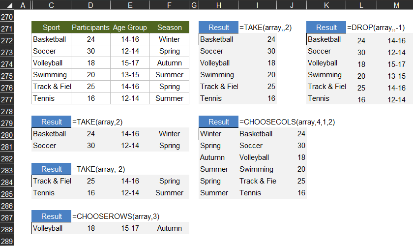
TAKE, DROP, CHOOSECOLS, CHOOSEROWS
=TAKE(array,rows,[columns])
=DROP(array,rows,[columns])
=CHOOSECOLS(array,col_num1,[col_num2],...)
=CHOOSEROWS(array,row_num1,[row_num2],...)
Use TAKE to extract a number of rows or columns from an array, either from the start or the end of the array. DROP is similar - but instead of extracting, it drops (removes) them. CHOOSECOLS lets you extract specific columns, and CHOOSEROWS lets you extract specific rows.
The main thing to remember is that TAKE and DROP work with n rows from the start or end of the array (not the middle). Use CHOOSEROWS and CHOOSECOLS for grabbing rows and columns out of the middle.
Keep in mind when using CHOOSECOLS and CHOOSEROWS that you do not need to list the columns and rows in a particular order. You can use these functions to change the order of the rows and columns in a very specific, non-sorted type way, such as column 4, 1, 3, 2.
The UNIQUE Function
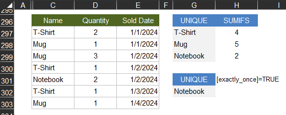
=UNIQUE(array,[by_col],[exactly_once])
UNIQUE is a useful function for returning the unique values in an array. The new list can be used to populate a drop-down selection or to help create a summary table to do something similar to pivot tables. You can set the [exactly_once] parameter to TRUE if you want only the values that appear exactly once.
FILTER, SORTBY, SORT
=FILTER(array,include,[if_empty])
=SORTBY(array,by_array1,[sort_order1],[by_array2],[sort_order2],...)
=SORT(array,[sort_index],[sort_order],[by_col])
FILTER lets you return a filtered set of results based on an include array, which is a set of TRUE/FALSE values, to specify which rows should be included.
SORTBY allows you to sort the array by the order specified in another array and you can include secondary sort criteria as well (sort by, then sort by, ...).
SORT lets you choose a specific column number to sort by. [sort-order] is 1 for ascending (default) or -1 for descending.
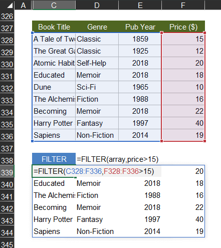
TIP When your table consists of named columns (either by creating named ranges or using structured table references), these functions are quite a bit easier to use. For example, =FILTER(tablename,price>15) is quite a bit easier to understand than =FILTER(C328:F336,F328:F336>15)
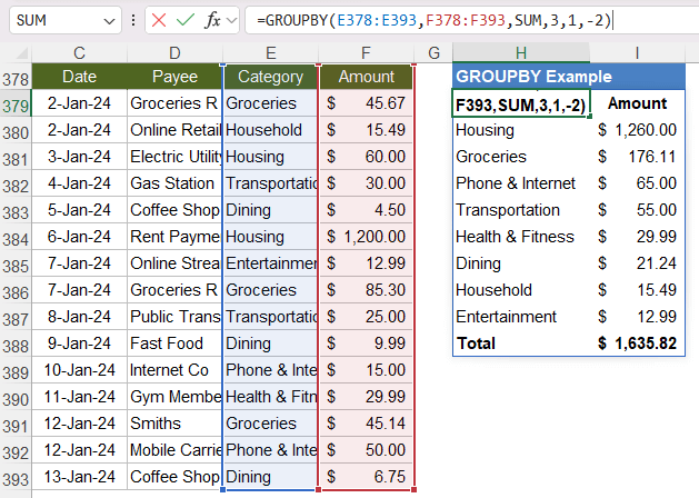
GROUPBY
=GROUPBY(row_fields, values, function, [headers], [totals], [sort_order], [filter_array])
This is one of the newer functions and it is extremely useful. You can use this function instead of a Pivot Table for a lot of things.
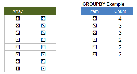
Get a Count of Each Unique Item
This is a common task in Excel Esport competitions, and it can be accomplished with a very simple GROUPBY formula. Note that the [sort_order] in this example is -2, meaning sort by the second column descending.
Here is an example formula you can try:
=LET(
    array,
      {"⚁","⚂","⚄","⚃";
       "⚁","⚂","⚂","⚀";
       "⚀","⚅","⚁","⚅";
       "⚄","⚂","⚁","⚂"},
    GROUPBY(TOCOL(array),TOCOL(array),ROWS,0,0,-2)
)
Result:
  { "⚂",5;
    "⚁",4;
    "⚀",2;
    "⚄",2;
    "⚅",2;
    "⚃",1 }
Summarize Expenses by Category
This is another useful example, for anyone wanting to analyze their personal finances: sum your expenses by category with a single simple function. This example helps me remember how to use GROUPBY. The "row_fields" parameter is the category you are grouping by and the "values" are the numbers you are counting or summing or averaging or whatever.
Other Array Functions
Although SEQUENCE is clearly my favorite function in this group, I use most of these functions frequently. You may note that I didn't even include the EXPAND function, because I haven't found a case where I've needed it yet.
Many (if not most) other functions can be considered dynamic array functions, such as TEXTJOIN, CONCAT, MMULT, TRANSPOSE, etc. because they allow you to use the # notation for defining an array reference and/or they can return a spillable array as the result. I limited this article to the newer functions that were specifically designed to work with this new type of dynamic array.
There are still plenty of functions that do not allow you to use an array as input (or you need to process an array by row or by column). This is where functions like BYROW, BYCOL can help.
For older examples of array functions, which now work as spillable arrays rather than CSE formulas, see Array Formula Examples.
References
support.microsoft.com: Dynamic Array Formulas and Spilled Array Behavior


Comments
Hello
As usual your Blog + Excel Workbooks are very comprehensive, you make it much more easily approachable with very useful generic helpful examples.
Question: Majority of what is described here is exclusively applicable to Office365.
Excel 2021, what are your suggestions for equivalents to:
TOCOL and/or VSTACK?
I’ve been using the LET formula, which until recently I’ve never heard of, was initially apprehensive of this, as looked lengthy, but it is coherent to edit such as:
=SORT(UNIQUE(LET(
a,B2#,
b,A2#,
ra,ROWS(a),
rb,ROWS(b),
rsq,SEQUENCE(ra+rb),
csq,SEQUENCE(,COLUMNS(a+b)),
out,IFS(rsq<=ra,INDEX(a,rsq,csq),rsq<=ra+rb,INDEX(b,rsq-ra,csq),TRUE,),out)))
You’re not going to like my answer, but my suggestion is to get Office365, if only so you can use the dynamic array formulas.