Dynamic Drop-Down Lists for Dates and Check Numbers

If you use Excel for money management or any type of activity where you are entering daily transactions or logging daily activities, then you may find it useful to create a dynamic drop-down list. This technique came about through the use of the Money Management template, so I will use that template as an example.

First, if you aren't familiar with how to use data validation to add an in-cell drop-down, read my article Create a Drop-Down List in Excel.

In the money management template, the Transactions worksheet provides a table for entering bank and credit card transactions, just like you would find in any check register or personal finance software. When we add new transactions, we want to be able to select the next date and next check number from a drop-down list as shown in the images below.

Dynamic drop-down list for Dates

Dynamic drop-down list for Check Numbers

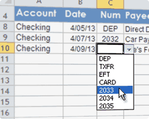
The list of dates includes the most recent date plus the dates for the next week. It would be much better if Microsoft provided a convenient built-in date picker tool, but this approach provides a useful substitute for now. We can still enter the date manually if we want to.

As you may know from your own experience, checks that you write are not always deposited in the order you write them. So, for the drop down list in the Num column, we can list the next three check numbers. (Note: after writing this article and creating these images, I found that I also wanted to list the previous two check numbers).

Setting up the Dynamic Drop-Down Lists

Step 1: Create the lists

The lists used for the dynamic drop-downs need a home, so for this example we can create a new worksheet and create the lists as shown in the image below. The formula in A6 is adding +1 to the current maximum check number in the Num column. Cell C2 is finding the most recent date in the Date column. The rest of the items in the list are just calculated from those two cells as shown.

Formulas for the drop down lists

Step 2: Name the lists

The next step is to name the ranges "num_list" and "date_list" by selecting the list (not including the header in row 1) and using the Name Box to name the ranges as shown in the next image.

Naming the lists

It isn't necessary to use named ranges when creating drop-down lists, but if you ever want to redefine the list, it's easier to redefine the named range than to update all the cells that use data validation to refer to the list. That brings us to the last step.

Step 3: Create the in-cell drop-downs

To set up the data validation drop-down lists, just select all of the cells in the Num column and go to Data > Data Validation, select List from the Allow field, and enter =num_list in the Source field, as shown in the image below. Do likewise for the Date cells to reference the date_list range.

Data Validation Settings

Something Really Fancy

One important thing to realize when creating dynamic drop-down lists is that the Source value must be a range reference. Even if you use a named range, it cannot be a formula like =A1:A10+2 which returns the values of the range. The reference CAN be a dynamic named range using OFFSET, INDEX, or INDIRECT.

So, let's say that I want the dates in a drop-down list to be ±5 days from the date that is currently in the cell. If the cell is empty, then I want it to be ±5 days from today's date.

To make this happen, you can create a helper worksheet (called "Dates") where column A:A is just a column of numbers 1:55000 formatted as dates (A1=1/1/1900, A2=1/2/1901, etc.), recognizing that the stored value for a date is simply a number (1/1/2017 is 42736).

Let's say you have a date stored in cell C8. Select cell C8 and go Formulas > Name Manager and create a named range "rel_date_list" using the following formula in the Refers To field (it is very important that C8 be a relative reference):

=INDEX( Dates!$A:$A, IF(C8="",TODAY(),C8)-5, 1 ):INDEX( Dates!$A:$A, IF(C8="",TODAY(),C8)+5, 1 )

Now, you can use =rel_date_list as the Source for a data validation drop-down list, and the list of dates in the drop-down will be ±5 days from the date in cell C8. Because you used a relative reference for the named range, you can copy/paste cell C8 to use this feature in other cells within the same worksheet.

When creating the named range, choose the current sheet as the Scope because after you create the name, the sheet name will automatically be added to the relative reference, and rel_date_list is only applicable to the worksheet where you defined it.