One of the most important tasks in personal finance is to keep a running balance of your checking and credit accounts, and spreadsheets are a common tool for doing that. In fact, tracking accounts is one of the original uses for the spreadsheet dating as far back as when the ancients etched ledgers on clay tablets.
The ancients may have occasionally made math errors when they recorded a running total or a running balance. We may think our modern spreadsheets are far superior because we let Excel formulas do the math for us, but we can run into other types of errors instead. The ability that Excel gives us to insert rows, delete rows, and move rows via cut and paste, can introduce hard-to-detect errors.
In this article, I'll explain the problems with the basic running balance formula and provide two robust solutions.
To see the examples in action, download the Excel file below.
Download the Example File (RunningBalance.xlsx)
This Article (bookmarks):
Problems with the Basic Running Balance
Consider the following very simple example showing deposits and withdrawals and a running balance. The basic running balance would be a formula that adds deposits and subtracts withdrawals from the previous balance using a formula like this: =SUM(D15,-E15,F14).
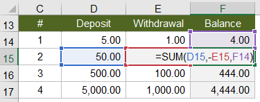
NOTE Why use SUM instead of =D15-E15+F14? Answer: The formula in the first row would lead to a #VALUE! error because of trying to add a text value (=5-1+"Balance"). The SUM function ignores text values. Another approach is to leave a blank row underneath the columns labels, or use the first row to enter the carry over balance instead of using a formula.
Problem #1: Deleting a Row Causes a #REF! Error

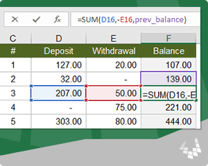
In this example, row 2 was deleted. The balance formula in row 3 now contains a #REF! error because the reference to the balance in row 2 was deleted. All dependent formulas also contain #REF! errors.
This error is very obvious, and can be fixed fairly easily by fixing the balance formula in row 3. While annoying to fix, it's not as scary as the errors that are harder to detect.
Problem #2: Inserting a Row Causes an Incorrect Running Balance

In this example, a new row was inserted above row 3 and the balance formula was then copied down. The problem is that the balance formula in row 3 is still referencing the balance from row 2.
The error checking feature in Excel was designed to help identify these types of errors. In this case, a little green triangle indicates an inconsistent formula. It isn't wise to rely on the error checking feature because it doesn't catch all errors.
Problem #3: Moving a Row Causes Hard-to-detect Errors
In this example, row 3 was cut and inserted above row 2. Are there any errors?

The scary thing about this example is that there is no obvious indicator of the errors. In fact, the running balance is wrong in both rows 2 and 3, because the formulas are not referencing the correct previous balance.
If I have an error in a spreadsheet, I would much rather see a glaring #VALUE! or #REF! error than have errors I can't see.
Design for Robustness to Common Usage
If you are designing a spreadsheet with a running balance, it's likely that you or somebody else may want to insert, delete, or move rows. So, you need to use formulas that don't cause hidden or hard-to-detect errors.
There are two fairly simple solutions for creating a robust running balance that don't break when you insert, delete or move rows.
Solution #1: Create a Running Balance using the OFFSET Function
The OFFSET function allows you to create a reference by specifying the number of rows and columns offset from a particular reference.
Syntax: =OFFSET(reference,rows,columns,[height],[width])
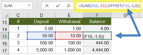
To refer to the previous balance, we can use the current balance (F15) as the reference and use -1 for the offset rows and 0 for the offset columns like this: =OFFSET(F15,-1,0). Nice and simple.
The OFFSET function does not directly reference cell F14, so if you delete row 14, no problem. You can insert, delete and move rows and the balance formula will always reference the cell above the current balance.
To see the OFFSET function used within functioning templates, take a look at the Checkbook Register and Credit Account Register, both of which include a running balance.
Pros:
OFFSET is compatible with Google Sheets and OpenOffice. The need for compatibility is one of the main reasons I use OFFSET in many of my templates. However, if you only use Excel, you might try Solution #2.
Cons:
OFFSET can make formulas difficult to understand. Notice that in the image above, the OFFSET formula highlights the reference (cell F15) rather than the cell that OFFSET refers to (cell F14).
OFFSET is a volatile function, which means it re-evaluates every time the worksheet is recalculated. This particular use is very efficient, so it likely won't cause a problem unless you have a lot of other inefficient formulas that depend on the results of the OFFSET formula.
Solution #2 - Create a running balance using a Relative Named Range
When you create a named range via Formulas > Define Name, you can use a relative reference like =F14 (no dollar signs) instead of an absolute reference like =$F$14. In this example, I've created prev_balance as a named range that refers to the cell immediately above the current balance.

The named range was created using a relative reference, so when the running balance formula is copied down, prev_balance will always refer to the cell immediately above the current cell, even if you insert, delete, or move the rows.
Not familiar with named ranges? Check out the references listed at the end of this article to learn more.
Pros:
Named ranges can make formulas easier to understand. Notice that unlike OFFSET, Excel highlights cell F14 (the cell that prev_balance is referring to).
Cons:
Most Excel users do not know how to use or create named ranges. Even advanced users may not know about relative named ranges. So, even though the formula may be easy to read, most people are not going to know why or how the formula works.
Named ranges have their own set of complexities and problems, especially when it comes to duplicating or moving worksheets.
Relative named ranges are not compatible with Google Sheets. Currently, Google Sheets treats all named ranges as absolute references (even though the references don't show dollar signs).
How to Create the Relative Named Range
This can be tricky. The most important step is the very first one: selecting the correct cell prior to defining the name.
- Select cell A2 or B2 or F2 or ZZ2 (any cell in row 2)
- Go to Formulas > Define Name
- Enter prev_balance in the Name field
- Set the Scope to the current worksheet
- In the Refers To field, enter =$F1 (no dollar sign before the 1)
In our example, the Balance is in column F, so we want prev_balance to always refer to column F. That is why we place a dollar sign in front of the F. It is also why it doesn't matter what cell in row 2 we choose in step 1.
Take it a Step Further: Create relative named ranges for deposit and withdrawal.
Although not necessary for making a robust running balance, you might be interested in making your formula even more readable, as shown in the image below.

The relative named ranges for deposit and withdrawal refer to columns D and E in the current row. To create these named ranges, follow similar steps as above, except enter =$D2 and =$E2 in the Refers to field for deposit and withdrawal.
NOTE If readable formulas is the goal, you might consider using Excel Tables with structured references.
Bonus Trick: Create a range named cell_above that works everywhere in the workbook
For the sake of being tricky, you could create a range named cell_above that always returns the cell in the previous row, anywhere you use it in the workbook.
- Select cell A2
- Go to Formulas > Define Name
- Enter cell_above in the Name field
- Set the Scope to Workbook
- In the Refers To field, enter =!A1 (no dollar signs, don't forget the exclamation mark)
A discussion of Scope is beyond the scope of this article, but the articles listed in the references below cover the topic well. Including the exclamation mark without the name of the worksheet is a trick I learned from Mynda Treacy that makes the relative named range work throughout the workbook.
Questions and Comments
If you have questions about how to apply these techniques or know of other ways they can be applied, feel free to comment below.
An example of another application would be to use OFFSET in the # column for sequential numbering that allows rows to be deleted without #REF! errors, like this: =1+OFFSET(current_cell,-1,0).
References
- Define and use names in formulas - support.microsoft.com - A good general overview of how to create and use named ranges.
- Relative Named Ranges - myonlinetraininghub.com - This is an excellent article about relative named ranges, including some very advanced uses.


Comments
Thanks for the detailed summary Jon. I like your relative named range solution.
Cheers,
Kevin Lehrbass
Just started using project planner template (excel version). Need to change the quarterly parameters. are you able to assist me please.
@Tim … will need more information. Please contact me via email on my Contact Us page.
I have a 2 week time sheet on a spreadsheet. I have a column to input comp time earned in that 2 week period and a column to input comp time used in that 2 week period. I have a beginning balance of accumulated comp time of 30 hours. I delete all the data and use the same time sheet for the next 2 week period. How can I add the earned comp time and subtract the comp time used from the beginning balance and keep this new beginning balance for the next 2 week period after deleting all the daily data from the previous 2 week period?
@John, you would first need to calculate the remaining comp time (end balance = beginning balance + total earned – total used). But, before you delete the data to start the new timesheet, you would need to enter the end balance into the beginning balance manually. Or, create a VBA macro to do it for you. Or, create multiple timesheet worksheets and link them together so that instead of deleting, you edit the next worksheet. Contact an Excel consultant (ExcelRescue.net) if you’d like something like that to be created for you.
Thanks so much for your article. As I’m using Google Sheets, I’m going to use the Offset function solution. The other thing i need to do is take the balance and transfer it to a master budget sheet. How can i do this if the cell that is shows the balance is changing with each line entry?
@Cathryn, Use a formula that will lookup the last value in the Balance column.
Hi,
Thank you for your excellent article.
Please have a look at the instructions in RunningBalance.xlsx under Create Relative Named Ranges for Deposit and Withdrawal and correct the entry for withdrawal Step 3.
You have: Step 3: Enter deposit in the Name field . I should be withdrawal which confused me slightly. I am using LibreOffice Calc and the line number is 123.
Hello.
I am using your checkbook register and love it! My question is, how do you copy and insert multiple lines in the register? I tried to copy several lines and insert them, but it doesn’t work. What am I doing wrong?
6 6
8 14
3 17
-2 15
I’d like a formula that creates a running balance in the total on the right. I want to format that column so every new number is added or subtracted from the previous balance. (eg: 6 + 8 = 14 for line 2) So no matter that numbers are added in the first column the running balance will show to the right. So simple. This seems impossible to find online. Everything is so complicated as if we’re doing the taxes for NASA.
The formula for a basic running balance is shown in the article: eg: F15=F14+E15 or F15=SUM(F14,E15)
Relative named range solution is awesome! With some IF statements, I was able to implement it within an Excel table (as opposed to range) and it worked very well. With tables, it’s always a problem referring to the previous row because of the nature of column references in tables. Thank you!
Does the formula work if there isn’t any figures in one of the cells? Ie line 15 withdraw has 15, deposit is left blank. Or vise versa? Thanks
It should work because a blank cell is treated as zero (0) if added or subtracted. But make sure it’s actually blank (no space characters which just make it appear blank)
Hello Steve, if a cell in your running balance formula is left blank, Excel treats it as zero, which means any subtraction or addition involving that blank cell would proceed as normal. To avoid issues, you can use the IFERROR function or similar logic to handle potential errors that arise from blank cells. Hope this helps!
Hello: Jon
Great Article!
Is there any way to create a Running Balance in Excel but in Pivot Table!?!
Worked very nicely for me in Libre Office with one exception:
the balance in the last row that is used propagates down to all the rows below.
It’s a bit ugly that way, but the thing that bothers me is watching the beachball while it saves the file. Is there some way to avoid this? thanks
Sorry. Not sure. I haven’t used OpenOffice or LibreOffice in a long time.
You are amazing! Thank you so much! I used this with amounts only in one column so I had to tweak it a little bit but I finally got it working! Thank you!