Template Support and FAQ
This page provides help related to getting started with Excel, problems downloading or accessing templates you've purchased, as well as some solutions to common Excel problems.
Although most of our templates are designed for people who know very little about Excel, the more you know about Excel, the more you will get out of our templates. For 140+ detailed tips and tutorials that can take you from beginner to proficient, see my new Spreadsheet Tips Workbook.
What type of help do you need?
Click on a topic below to learn more.
- New to Spreadsheets?Templates can make you a powerful Excel user, but learning the basics is important.
-
Problems Downloading, Opening, Saving
Don't know what to do with a ZIP file? Is your firewall preventing downloads? -
Solutions to Common Template Issues
How to add rows, define the print area, change formatting, and other common issues -
Help with Gantt Chart Pro
Questions about purchasing? Other technical issues? -
Other Questions About Specific Templates?
What you need to tell us before we can be any help.
Need help customizing a spreadsheet?
ExcelRescue is a Vertex42 Approved consultancy, meaning that can help you edit, fix and customize Vertex42 spreadsheets. Their system allows them to take on both small and large tasks. They have a simple online form for submitting tasks and a very reasonable pricing structure.
Learn more about ExcelRescue.net >
Basic Spreadsheet Terminology
To use Vertex42's templates, you will want to at least become familiar with basic spreadsheet terminology. Otherwise, you won't be able to understand instructions.
The screenshot below shows an Excel 2010 workbook named My_Workbook.xls. A spreadsheet file (extensions .xls, .xlsx, .ods) is called a workbook. A workbook may contain one or more worksheets, shown as tabs at the bottom of the window. Each worksheet is made up of cells in a rectangular grid. The rows are numbered. The columns are labeled with letters. A group of cells is called a range.
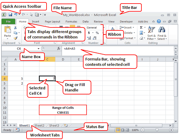
In the image above, cell C4 is currently selected. The Formula Bar is showing that cell C4 contains a formula, which you can identify because it starts with an equal sign (=). The formula is adding the values found in cells A4 and A5.
Almost everything else you need to know about Excel to use our spreadsheet templates is explained in Microsoft's own getting started guide found online or in Excel's Help system.
Excel Tutorials for Students
Check out our Excel Tutorials page for a number of free video tutorials that teach students the basics of using a spreadsheet and how to create various types of charts.
Review the Training on the Microsoft Site
Most of our templates are designed for spreadsheet users who at least know the basics, so please review the getting started material on support.office.com.
Basic Excel Training - Videos and resources for getting started
- Article: Basic tasks in Excel
Excel 2013
- Video: Start Using Excel
Excel 2010 or Older: Use Excel training for newer versions and adapt the best you can (and definitely consider upgrading).
Critical stuff to know ...
- Common spreadsheet terminology (see above)
- How to open and save files
- How to enter and edit data (i.e. type in cells, the formula bar, etc.)
- How to format cells and text
- How to recognize and use basic formulas
- How to print and change print settings
- How to use conditional formatting
Other useful articles/videos/training on microsoft.com
Using Google Sheets?
Google Sheets is quickly becoming a very useful alternative to Excel, especially if you are mainly using basic features or if you are using it for collaboration.
Learn the basics of Google Drive and important basic spreadsheet skills by watching the new video tutorial on our YouTube channel:
► Google Sheets - Easy Beginner's Guide
I Purchased a File, but Can't Download - or -
I Need to Return to the Download Page
If you had a problem downloading or need to re-download your file(s) or want to download an updated version, use the following link to get back to the download page.
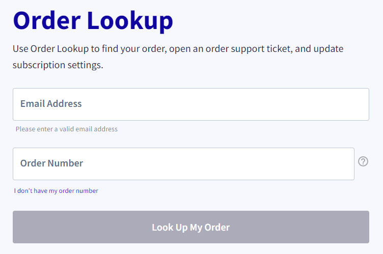
After you get go to www.clikbank.com, you should see the following Order lookup form:
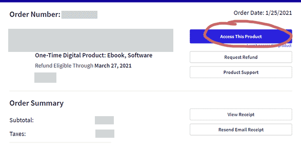
After submitting and verifying your order information (receipt # and email), look for the Access This Product button as shown in the image below:
If the Access This Product button doesn't work (does nothing), check to make sure your browser hasn't blocked pop-ups - because this link opens in a new window.
Note: Your email receipt also contains a link that can take you back to the download page.
I got to the download page, but still can't download ...
We can only guess unless you give us specific information. You may have a firewall that prevents downloading spreadsheet files, your browser might be blocking javascript, etc. In these cases, contact us with your receipt # and the name of the product you purchased, and we can send you the files via email.
When contacting us, please give us specific details about why you are unable to download. Do you click on a link and nothing happens? Are you sent to an error page? Does a message pop up giving an error? If you can give us more information, then we can work on making the process more robust. Thank you.
For more information about the process for downloading purchased files, particularly the Gantt Chart Template, please see our FAQ for Purchasing article.
I Can't Open a Downloaded File
Make sure you are using the right software for the type of file you have downloaded. Vertex42 download files have one of the following extensions in the file name:
- .XLS - an Excel 97-2003 Workbook file
- .XLSX - an Excel 2007+ Workbook file
- .ZIP - a common file format for compressing large files and combining multiple files in a single download. See below for how to extract a .zip file.
- .ODS - a spreadsheet file format for OpenOffice.org Calc
- .DOC - a document file for Microsoft Word
- .PDF - not a spreadsheet, but let's assume you know that already
I'm Unable to Download a Free Template
If you have a firewall the blocks your ability to download spreadsheet files from the internet, then please talk with your system administrator. There isn't much we can do about that problem. If you don't think this is the problem, please contact us and provide as many details as you can about the problem.
I Can't Find the File I Downloaded
Save (not Open): When you download a file, save it to your computer then open it using the correct software (unless it is a .ZIP file - see below for that). You may get a window asking whether you want to Save or Open the file. Click on SAVE! If you click on Open, your browser may try to open the spreadsheet or file inside the browser.
Can't find the file after downloading? Look on your Desktop, your My Downloads directory, or your default Downloads directory. If you know the filename of the file you are downloading, that will help you know whether to look for a .XLS file or a .ZIP file.
How do I Extract .ZIP Files
A file with a .zip extension is called a ZIP file and is simply a way of either compressing a file (to make it a smaller size for faster download) or archiving multiple files into a single file. Vertex42 uses .zip files for both of these reasons.
You must extract spreadsheet files from a .zip file before opening them, or the spreadsheets will open as "Read-Only", preventing editing or saving. So, even though you might be tempted to double-click on a file from within the .zip folder, don't do that - first extract the .zip file.
I Can't Edit or Change Values in the Spreadsheet
When a file is downloaded from the internet, Excel 2010/2013/2016 will usually open the file in "[Protected View]" and a message bar will be shown at the top similar to the one in the image below. To edit the file, you'll need to click on the "Enable Editing" button. In Excel 2016, click on "Click for more details" and then click on "Edit Anyway."
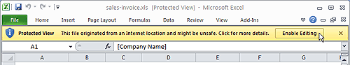
For more information about Protected View, see "What is Protected View?" at support.office.com.
If you are getting the message "Office has detected a problem with this file," please email vertex42 and report the exact name of the file that you downloaded. Most likely, the file is just damaged or Office is incorrectly reporting a problem (especially newer versions of Excel opening older files). If you are using Excel 2010 or later, download the .XLSX files instead of .XLS files.
In Excel 2016, some people are reporting problems with warnings similar to this or with messages about files being corrupt. Try going to the Excel Trust Center Settings and adding the location of your downloaded templates to Trusted Locations.
Excel is telling me I need to enter a password
Some Vertex42 templates are provided as free trials, with some cells and features "locked" by using password protected worksheets. When attempting to change a locked cell, you may get the following message:
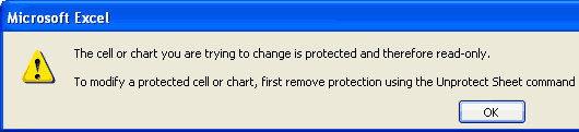
If you follow the instructions in that message and attempt to Unprotect the sheet, you may be asked for a password. When a worksheet is in Protected mode you will also see some commands in the menu disabled.
Vertex42.com uses password protected worksheets as a means of allowing customers to try a spreadsheet and use some limited features before buying an "unlocked" version.
Note: On Vertex42.com, all files that are purposely password protected in this way have "_L" in the name of the file, such as gantt-chart_L.xls.
File Opening in [Read-Only] Mode
One of the most common questions I get from people is "I can't edit the spreadsheet and save my changes". That is not a very helpful way to report a problem, but most of the time the cause is either:
- The file was opened in a browser rather than in Excel (see the section above titled "I Can't Find the File I Downloaded")
- The file was not extracted from the .zip file before opening (see the section "How do I Extract .ZIP Files").
If you already have another copy of the file open, Excel will ask if you want to open as read-only. If you are SURE that you do not have another copy of the file open, then Windows is probably just really confused (it gets like that sometimes) and you may need to restart your computer.
File Opening in [Compatibility] Mode
If you open a .XLS file using Excel 2007+, it will open the file in [Compatibility] Mode. There are many features in the newer versions of Excel that are not backward compatible with Excel 2003. Excel tries to warn you when you use features that are not compatible, but you only find out what is NOT compatible after trying to SAVE your file.
So, if you are using Excel 2007+ and you do not need to share your file with anybody who is using Excel 2003 or earlier, you can choose to save your file as a .XLSX file to avoid having to deal with the Compatibility messages.
Changing the Currency Symbol
Many Vertex42 templates are financial in nature and usually display the dollar currency symbol "$" by default. To change the symbol, select the cell and then press Ctrl+1 or go to Format > Cells to open the Format Cells dialog box. In the Number tab, select Currency in the Category list. Then select your desired currency symbol from the Symbol drop-down box.
Fixing Cells that Display "#######"
If you see "#######" in a cell, it means that the column is not wide enough to display the contents of the cell. Just increase the column width or decrease the font size to fix this problem.
Worksheets Appear to be Missing
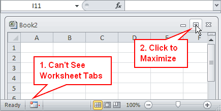
Many of the Vertex42 templates include workbooks with multiple worksheets. I get a lot of email from people saying they can't find the other worksheets. The problem is almost always that they downloaded the wrong file or the inner Excel workbook window is not maximized.
If you look at the bottom of your Excel window and do not see worksheet tabs, then click on the Maximum button as shown in the image below:
Getting Rid of the Green Triangles (Error Checking)
One of the most annoying features in Excel (in my opinion) is the background error checking feature, which adds little green triangles to cells for various reasons, such as if a formula refers to an empty cell or if Excel thinks a formula is inconsistent. Many of these types of warnings are NOT errors, especially not when done intentionally as in the calendar template shown below.
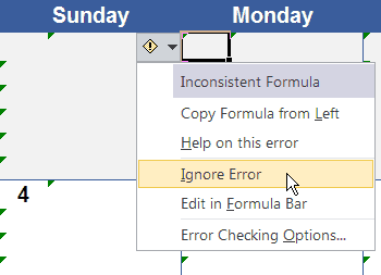
If you are annoyed by the green triangles, you can click on the [!] box and choose "Ignore Error" to make the green triangle go away, or you can click on Error Checking Options to get to the window shown below. You can also get to these options by going to File > Options.
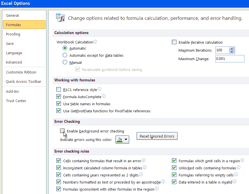
Uncheck the "Enable background error checking," or uncheck just the rules that are the most annoying, such as "Formulas referring to empty cells" and "Formulas inconsistent with other formulas in the region".
Adding Rows to an Invoice, Budget category, etc.
Many of the Vertex42 templates are designed to allow you to add and delete rows as need such as invoices, budget templates, checkbook registers, exercise logs, etc. The important thing to remember is that when you add a row, you not only need to insert the row, but you also need to (1) copy the formulas and formatting and (2) ensure that subtotal formulas and chart series expand to include the new row. To help ensure that this happens follow these steps:
Method 1: Insert a Blank Row and Then Copy Formulas- Select any row in the table EXCEPT for the first row of the table or sub-section: Click on the row number or press Shift+Space.
- Insert a new row above the currently selected row: Press Ctrl+Shift++ -or- right-click on the row number and select Insert -or- use the menu to go to Insert > Rows.
- Copy the formulas and formatting: With the new row currently highlighted, press Ctrl+d to copy the formulas and formatting from the row immediately above the current one.
- Make any necessary changes to the newly inserted row.
- Select a row you want to copy: Click on the row number or press Shift+Space.
- Copy the row: Press Ctrl+c.
- Select any row in the table EXCEPT for the first row of the table or sub-section: Click on the row number.
- Insert the copied row: Press Ctrl+Shift++ -or- right-click on the row number and select Insert Copied Cells.
- Make any necessary changes to the newly inserted row.
Method 2 is used extensively in the gantt chart template. It is also handy if you are using the checkbook register, where you may have recurring bills. You can select and copy the group of rows, insert those copies rows at the end, and then just change the dates.
If the template uses subtotals or charts, you must insert copied rows ABOVE the last row or BELOW the first row (or somewhere in between).

Redefining the Print Area
Defining the Print Area: Sometimes you will want to print a specific area of the spreadsheet, or you may need to redefine the print area that is already set. To do this ...
- In Excel 2007-2019: Select the Range you want to print, then go to Page Layout > Print Area > Set Print Area.
- In Excel 2003: Select the Range you want to print, then go to File > Print Settings > Set Print Area.
Scaling the Page: After you define the print area, you can tell Excel to fit the area on a single page or multiple pages. To do this, open up the Page Setup dialog box, go to the Page tab, then set the Scaling as needed. When fitting the print area to a number of pages, leave one of the numbers off. Excel will find the best fit for the other direction.
- In Excel 2007-2019: Go to Page Layout and click on the little arrow to the right of Page Setup.
- In Excel 2003: Go to File > Page Setup
Editing Date Formats for Your Country/Language
Most Vertex42 templates use English date formats, specifically U.S. formats. If you want to use a different date format, such as d/m/yy instead of m/d/yy or if you want to display the month or day of the week in a different language, you can create or modify the custom date format used in the template.
The following is a very good article on working with custom date formats: "How to change date formats in Excel and create custom formatting" on ablebits.com.
Finding Your Locale Code: If you want to use a locale code like [$-409] in your date format string, you can look for your locale code in the LCIDHex column of This List of Locale Codes. For example, the LCIDHex code is "0c0c" for French_Canadian, so you can use a custom date format code of "[$-0c0c]dddd, mmmm d, yyyy" to show day and month names in French.
If you are new to Excel, or are having problems using the template, please see the information in the previous two sections on this page. For questions more specifically about the Gantt Chart Template, see the following two articles:
For other questions, contact us.
How do I return to the download page?
If you had a problem downloading or need to re-download your file(s) or want to download an updated version, log in to clickbank.com using the following link to get help with your order.
After submitting and verifying your order information (receipt # and email), look for the Access This Product button as shown in the image below:
Note: Your email receipt also contains a link that can take you back to the download page.
◄ Return to the Gantt Chart Pro page
For questions or problems related to Vertex42 templates, you are welcome to contact us via email, especially if it concerns an error or bug in a spreadsheet. If you need assistance customizing a spreadsheet, you may want to contact an excel consultant to request a quote. For general Excel questions (such as questions about how to use Excel rather than errors in a Vertex42 template), please try using Google to find an answer or ask your question on an Excel help forum.
Please be as descriptive as possible when explaining the problem you are having. Also, courtesy and politeness are greately appreciated.
If you need help with a template, it is critical that you tell us ...
- The version of Microsoft Excel you are using (Excel 2003, 2004(Mac), 2007, 2008(Mac), 2010, 2011(Mac), 2013, 2016, 2019, or Excel 365. If you aren't using Excel, please tell us what you ARE using.
- The exact filename of the file you downloaded (e.g. 2022-calendar.xlsx)
- As much detail about the problem as you can provide. Screenshots (images of your Excel window) are extremely helpful in communicating your problem.