Generating Random Numbers using Excel
[ Step 1: Sales Forecast Model ] ![]()
![]() [ Creating a Histogram in Excel ]
[ Creating a Histogram in Excel ]
Step 2: Generating Random Inputs
The key to Monte Carlo simulation is generating the set of random inputs. As with any modeling and prediction method, the "garbage in equals garbage out" principle applies. For now, I am going to avoid the questions "How do I know what distribution to use for my inputs?" and "How do I make sure I am using a good random number generator?" and get right to the details of how to implement the method in Excel.
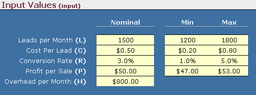
For this example, we're going to use a Uniform Distribution to represent the four uncertain parameters. The inputs are summarized in the table shown below. (If you haven't already, Download the example spreadsheet).

Figure 1: Screen capture from the example sales forecast spreadsheet.
The table above uses "Min" and "Max" to indicate the uncertainty in L, C, R, and P. To generate a random number between "Min" and "Max", we use the following formula in Excel (Replacing "min" and "max" with cell references):
You can also use the Random Number Generation tool in Excel's Analysis ToolPak Add-In to kick out a bunch of static random numbers for a few distributions. However, in this example we are going to make use of Excel's RAND() formula so that every time the worksheet recalculates, a new random number is generated.
Let's say we want to run n=5000 evaluations of our model. This is a fairly low number when it comes to Monte Carlo simulation, and you will see why once we begin to analyze the results.
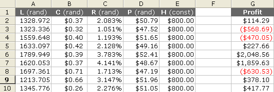
A very convenient way to organize the data in Excel is to make a column for each variable as shown in the screen capture below.

Figure 2: Screen capture from the example sales forecast spreadsheet.
Cell A2 contains the formula:
=Model!$F$14+RAND()*(Model!$G$14-Model!$F$14)
Note that the reference Model!$F$14 refers to the corresponding Min value for the variable L on the Model worksheet, as shown in Figure 1. (Hopefully you have downloaded the example spreadsheet and are following along.)
To generate 5000 random numbers for L, you simply copy the formula down 5000 rows. You repeat the process for the other variables (except for H, which is constant).
Step 3: Evaluating the Model
Our model is very simple, so to evaluate the output of our model (the Profit) for each run of the simulation, we just put the equation in another column next to the inputs, as shown in Figure 2.
Cell G2 contains the formula:
=A2*C2*D2-(E2+A2*B2)
Step 4: Running the Simulation
To iteratively evaluate our model, we don't need to write a fancy macro for this example. We simply copy the formula for profit down 5000 rows, making sure that we use relative references in the formula (no $ signs). Each row represents a single evaluation of the model, with columns A-E as inputs and the Profit as the output.
Re-run the Simulation: F9
Although we still need to analyze the data, we have essentially completed a Monte Carlo simulation. We have used the volatile RAND() function. So, to re-run the entire simulation all we have to do is recalculate the worksheet (F9 is the shortcut).
This may seem like a strange way to implement Monte Carlo simulation, but think about what is going on behind the scenes every time the Worksheet recalculates: (1) 5000 sets of random inputs are generated (2) The model is evaluated for all 5000 sets. Excel is handling all of the iteration.
If your model is not simple enough to include in a single formula, you can create your own custom Excel function (see my article on user-defined functions), or you can create a macro to iteratively evaluate your model and dump the data into a worksheet in a similar format to this example (Update 9/8/2014: See my new Monte Carlo Simulation template).
In practice, it is usually more convenient to buy an add-on for Excel than to do a Monte Carlo analysis from scratch every time. But not everyone has the money to spend, and hopefully the skills you will learn from this example will aid in future data analysis and modeling.
[ Step 1: Sales Forecast Model ] ![]()
![]() [ Creating a Histogram in Excel ]
[ Creating a Histogram in Excel ]
A Few Other Distributions
My new Monte Carlo Simulation template includes a worksheet that calculates inputs sampled from a variety of distributions. Some of the formulas are listed below.
Normal (Gaussian) distribution
To generate a random number from a Normal distribution you would use the following formula in Excel:
Ex: =NORMINV(RAND(),$D$4,$D$5)
Excel 2010+: =NORM.INV(RAND(),$D$4,$D$5)
Lognormal distribution
To generate a random number from a Lognormal distribution with median = exp(meanlog), and shape = sdlog, you would use the following formula in Excel:
Ex: =LOGINV(RAND(),$D$6,$D$5)
Excel 2010+: =LOGNORM.INV(RAND(),$D$4,$D$5)
Weibull distribution
There isn't an inverse Weibull function in Excel, but the formula is quite simple, so to generate a random number from a (2-parameter) Weibull distribution with scale = c, and shape = m, you would use the following formula in Excel:
Ex: $C$5*(-LN(1-RAND()))^(1/$C$6)
Beta distribution
This distribution can be used for variables with finite bounds (A,B). It uses two shape parameters, alpha and beta. When alpha=beta=1, you get a Uniform distribution. When alpha=beta=2, you get a dome-shaped distribution which is often used in place of the Triangular distribution. When alpha=beta=5 (or higher), you get a bell-shaped distribution. When alpha<>beta (not equal), you get a variety of skewed shapes.
MORE Distribution Functions: Dr. Roger Myerson provides a free downloadable Excel add-in, Simtools.xla, that includes many other distribution functions for generating random numbers in Excel.
