Grouping and Outlining in Excel
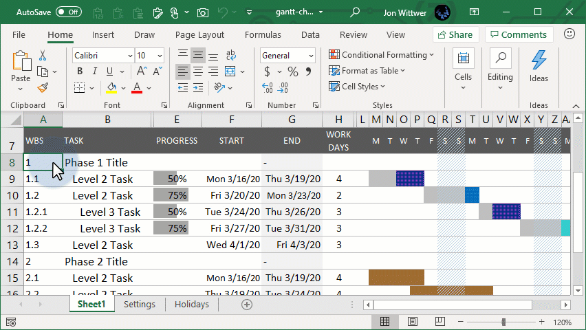
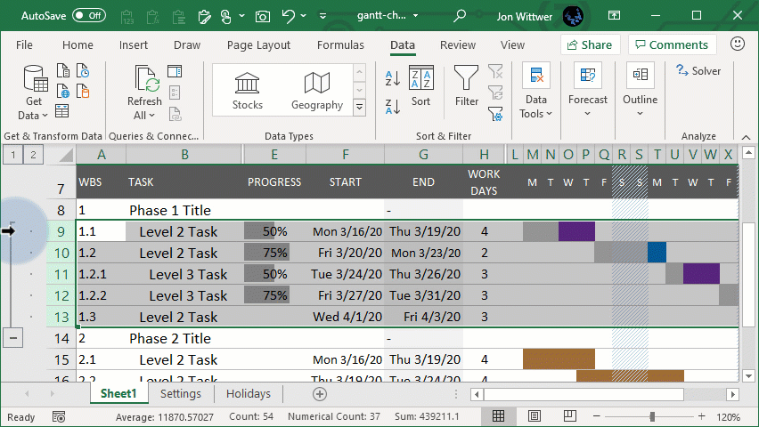
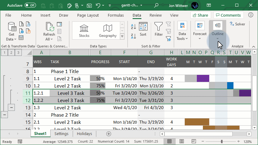
Grouping rows in Excel allows you to easily expand or collapse rows by clicking on a +/- button. This is especially useful for groups of tasks in a gantt chart and other types of hierarchical lists where you may want to toggle certain rows on/off. In this article, I'll explain how to use the Group and Outline feature using a simple gantt chart as an example.
How to Group Rows in Excel
Step 1: Select the rows that you want to hide when the button is clicked.
Step 2: Go to Data > Outline > Group
How to Hide/Show Outline Symbols
If for some reason the outline symbols do not show up when you use this feature, your worksheet may have the symbols hidden via the worksheet settings. To hide/show outline symbols in a specific worksheet, follow these steps:
Step 1: Go to File > Options > Advanced
Step 2: Scroll down to the "Display Options for This Worksheet"
Step 3: Check or Uncheck the "Show outline symbols if an outline is applied"
How to Group Rows Using a Keyboard Shortcut
Use the keyboard shortcut Shift+Alt+⇨ (Right Arrow Key) to Group rows more quickly, especially if you need to create multiple groups of rows. To Ungroup, you can use the keyboard shortcut Shift+Alt+⇦ (Left Arrow Key).
How to Move the Expand/Collapse Buttons to the Top of the Groups
I find that it makes more sense to have the toggle buttons at the top of each group. That is a workbook setting that you can change by following these steps:
Step 1: Go to Data > Outline and click on the outline settings button in the lower right corner.
Step 2: Uncheck the "Summary rows below detail" box.
Adding Outline Numbering in Excel
Outlining with Manual Numbering
You can create manual outline numbering such as 1, 1.2, 1.2.3, etc. by converting the cells used for the outline numbers to text. If the number of items will never be greater than 9, you can use a custom number format such as #.#.#.# to display 4.234 as 4.2.3.4.
The problem with manual outline numbering is that when you make a change, you may need to manually change all the rest of the numbers in the outline.
Outlining with Automatic Numbering
The Work Breakdown Structure (WBS) numbering system used for project schedules and Gantt charts uses a numbered outline where # is a first-level task, #.# is a second-level task, #.#.# is a third-level task, etc.
If you never have more than 9 tasks within a given level, then you could use a custom number format #.#.# to display 2.34 as 2.3.4 and then you could just add 0.01 to the next task to get 2.35 which would display as 2.3.5.
To prevent reference errors when inserting or deleting rows, you can use the OFFSET function to increment the outline number (see the example in my article Volatile Functions - What's the Big Deal).
If you could end up with more than 9 items in a given level within your outline, the formula gets a lot more complicated. One solution to this problem would be to use a custom VBA function (see the reference below). However, it IS possible to do this without VBA or macros, as I have done with the formulas I created for the gantt chart template. I'm not going to explain the formula in detail, because in the gantt chart template all you have to do is copy the row with the formula that you want to use (there are different formulas for Level 1, Level 2, Level 3, etc.) and everything will work out.
If you simply MUST know how the formula works, then I'll just give you a place to start: The key is to use the SUBSTITUTE() function to replace a period "." with some other character and then use the FIND() function to locate the position of that character with the text.