L_SLICE
=L_SLICE(array, row_start, row_end, [col_start], [col_end])
| Argument | Description | Example |
|---|---|---|
| array | A range of values (numbers or text) | |
| row_start | (default=1) The index of the first row to include | 2 |
| row_end | (default=last) The index of the last row to include | 4 |
| col_start | (default=1) The index of the first column to include | 1 |
| col_end | (default=last) The index of the last column to include | 3 |
Description
The L_SLICE function for Excel is based on the Javascript slice() function which allows you to return a subset of values from an array by specifying a start and end index. The Excel function permits you to do retrieve a horizontal slice (a range of rows) and a vertical slice (a range of columns) simultaneously. This results in a method for retrieving a block or submatrix based on specifying the start and end indices.
Like other Excel functions, the indices of an array start at 1. If the specified index values are negative, then they represent counting backward from the last value in the array. For example, a column index of -2 is the second-to-last column.
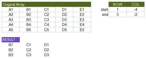
Example:
=LET(
    array, {"A","B","C","D","E"}&{1;2;3;4;5},
    L_SLICE(array,1,3,-4,-2)
)
Using Built-in Excel Functions
When the index values are positive, the behavior of the L_SLICE function can be achieved through a number of different methods using built-in Excel functions. Perhaps the most elegant is the INDEX():INDEX() formula.
Using OFFSET:
=OFFSET(INDEX(array,1,1),row_start-1,col_start-1,row_end-row_start+1,col_end-col_start+1))

Using DROP & TAKE:
=DROP(TAKE(array,row_end,col_end),row_start-1,col_start-1)

Using INDEX():INDEX()
=INDEX(array,row_start,col_start):INDEX(array,row_end,col_end)

Using CHOOSEROWS & CHOOSECOLS
[See the function code below]
Some of these formulas return errors if row_end > ROWS(array) or col_end > COLUMNS(array). L_SLICE was designed to be more robust and also to allow negative values for the indices.
Lambda Formula
This code for using L_SLICE in Excel is provided under the License as part of the LAMBDA Library, but to use just this function, you may copy the following code directly into your spreadsheet.
Code for AFE Workbook Module (Excel Labs Add-in)
/**
* Return a subset of rows and columns from an array
*/
L_SLICE = LAMBDA(array,row_start,row_end,[col_start],[col_end],
LET(doc,"https://www.vertex42.com/lambda/slice.html",
    rows,ROWS(array),
    cols,COLUMNS(array),
    row_start,IF(ISBLANK(row_start),1,
        IF(row_start>0,IF(ABS(row_start)>=rows,1,rows+row_start+1),row_start)
    ),
    row_end,IF(OR(ISBLANK(row_end),row_end>rows),rows,
        IF(row_end>0,IF(ABS(row_end)>=rows,1,rows+row_end+1),row_end)
    ),
    col_start,IF(ISBLANK(col_start),1,
        IF(col_start>0,IF(ABS(col_start)>=cols,1,cols+col_start+1),col_start)
    ),
    col_end,IF(OR(ISBLANK(col_end),col_end>cols),cols,
        IF(col_end>0,IF(ABS(col_end)>=cols,1,cols+col_end+1),col_end)
    ),
    new_array,CHOOSEROWS(array,SEQUENCE(row_end-row_start+1,,row_start,1)),
    CHOOSECOLS(new_array,SEQUENCE(col_end-col_start+1,,col_start,1))
));
Named Function for Google Sheets
Name: L_SLICE
Description: Return a subset of rows and columns from an array
Arguments: array, row_start, row_end, col_start, col_end
Function:
[Same as Excel version]
The Excel version was designed so that it would work in Google Sheets
