SIMPSON
=SIMPSON(y, [x], [dx])
| Argument | Description | Example |
|---|---|---|
| y | A column vector of y values | {0;1;4;9;16} |
| x | (optional) A column vector of x values | {0;1;2;3;4} |
| dx | (default=1 if x is blank) Used to specify uniform spacing if x is omitted | 1 |
In the template file, navigate to the Calc worksheet to see the SIMPSON function in action.
Description
SIMPSON is an implementation of the composite Simpson's 1/3 Rule for numerical integration of irregularly spaced data. You would use it when you want higher accuracy than the trapezoidal rule, but you still only have a set of (x,y) points rather than the ability to evaluate the function at more points.
The following image shows a set of 8 points. The black line is the actual curve which for this particular example is the function \(f(x)=0.5x^3+5x^2-10x+10\). The composite Simpson's 1/3 Rule estimates the area under the curve between each subsequent set of 3 points (The "1/3" in the name of the rule comes from the resulting formula, not the fact that it uses 3 points).
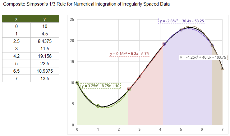
Simpson's 1/3 Rule can be derived from a quadratic polynomial fit over 3 points and integrates the quadratic polynomial to find the area under the curve for the interval \([x_i,x_{i+2}]\). In the above example, the first area is shown as light green over the interval \([0,2.5]\), and the quadratic polynomial fit is \(y=3.25x^2-8.75x+10\). The green area is estimated as \(\int_0^{2.5}3.25x^2-8.75x+10dx=14.58333\). It is an estimate because the quadratic fit may not exactly fit the true curve over this interval, even though we can exactly integrate a quadratic polynomial.
The red and purple areas for intervals \([2.5,4.2]\) and \([4.2,6.5]\) are calculated in turn.
If there is an even number of points like this example, the final area (shown as light brown) is calculated by using a quadratic fit of the last 3 points but integrating only over the final interval \([x_{N-1},x_N]=[6.5,7]\).
The SIMPSON function uses the formulas provided in references [1-3] rather than using POLYFIT and POLYINT. Aside from machine precision error, the results are the same as using POLYFIT and POLYINT, but with greater efficiency. Higher-order Newton-Cotes formulas (the Trapezoidal Rule being 1st-order and Simpson's 1/3 Rule being 2nd-order) can be implemented using POLYFIT and POLYINT.
Uniformly Spaced Points
If the x values are uniformly spaced, you can omit the x parameter and specify the value for dx=Δx where \(h={\Delta}x\) is constant. With a constant h spacing, the formulas for Simpson's 1/3 Rule are simplified to:
$$ \int_{x_i}^{x_{i+2}}f(x)dx \approx \frac{1}{3}h(f(x_i)+4f(x_{i+1})+f(x_{i+2})) $$The formula for the final area if there are an even number of points simplifies to:
$$ \int_{x_{N-1}}^{x_N}f(x)dx \approx \frac{1}{3}h(\frac{5}{4}f(x_N)+2f(x_{N-1})-\frac{1}{4}f(x_{N-2})) $$Cumulative Integration
I have not implemented a cumulative option for SIMPSON like with TRAPZ or PPINT because the function does not produce a result for each corresponding value of y (the integration occurs over 3 points rather than just 2).
With some limited experimentation, I have found that integrating a cubic spline using PPINT and CSPLINE can produce results with approximately the same order of error as SIMPSON when PDIFF(x,y,1,3) is used to estimate the slopes for CSPLINE. More rigor in the derivation of the error would be needed to further test this.
Lambda Formula
This code for using SIMPSON in Excel is provided under the License as part of the LAMBDA Library, but to use just this function, you may copy the following code directly into your spreadsheet.
Code for AFE Workbook Module (Excel Labs Add-in)
/**
* Numerical Integration using Composite Simpson's 1/3 Rule
*/
SIMPSON = LAMBDA(y,[x],[dx],
LET(doc,"https://www.vertex42.com/lambda/simpson.html",
    dx,IF(ISOMITTED(dx),1,dx),
    n,ROWS(y),
    integral,REDUCE(0,SEQUENCE(INT((n-1)/2),1,1,2),LAMBDA(acc,i,
        IF(ISOMITTED(x),
            acc+(1/3*dx*(INDEX(y,i)+4*INDEX(y,i+1)+INDEX(y,i+2))),
            LET(
                h_1,INDEX(x,i+1)-INDEX(x,i),
                h_2,INDEX(x,i+2)-INDEX(x,i+1),
                area,(h_1+h_2)/6*(
                    (2-h_2/h_1)*INDEX(y,i) +
                    (h_1+h_2)^2/(h_1*h_2)*INDEX(y,i+1) +
                    (2-h_1/h_2)*INDEX(y,i+2)),
                acc+area
            )
        )
    )),
    lastinterval,IF(ISODD(n),0,
        IF(ISOMITTED(x),
            dx*(5/12*INDEX(y,n)+2/3*INDEX(y,n-1)-1/12*(INDEX(y,n-2))),
            LET(
                h_1,INDEX(x,n)-INDEX(x,n-1),
                h_2,INDEX(x,n-1)-INDEX(x,n-2),
                alpha,(2*h_1^2+3*h_1*h_2)/(6*(h_2+h_1)),
                beta,(h_1^2+3*h_1*h_2)/(6*h_2),
                nu,(h_1^3)/(6*h_2*(h_2+h_1)),
                alpha*INDEX(y,n)+beta*INDEX(y,n-1)-nu*INDEX(y,n-2)
            )
        )
    ),
    integral+lastinterval
));
Named Function for Google Sheets
Name: SIMPSON
Description: Numerical Integration using Simpson's 1/3 Rule
Arguments: y, x, dx
Function:
[in the works]
SIMPSON Examples
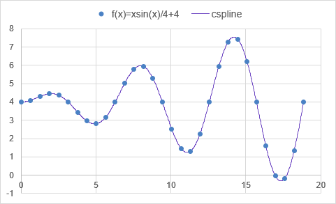
The following is the result of using SIMPSON for the same 31 points as in the PPINT example:
=LET(
    xs, LINSPACE(0,6*PI(),31),
    ys, xs/4*SIN(xs)+4,
    SIMPSON(ys,xs)
)

Result: 70.681554
Error:  -0.004280
Note: The trapezoidal rule using TRAPZ for these same 31 points results in 70.8419 with an error of 0.156.
See Also
DIFF, FDIFF, PDIFF, TRAPZ, SIMPSON
- [1] Wikipedia: Simpson's rule
- [2] Shklov, N. (Dec 1960), "Simpson's Rule for Unequally Spaced Ordinates", The American Mathematical Monthly, 67 (10): 1022–1023, doi:10.2307/2309244
- [3] Cartwright, K.V. (Sep 2017), "Simpson's Rule Cumulative Integration with MS Excel and Irregularly-spaced Data (pdf)", Journal of Mathematical Sciences and Mathematics Education, 12 (2): 1–9
- Wikipedia: Numerical Integration
- Wikipedia: Newton-Cotes formulas
- SciPy - simpson function
