EIGENVALUE
=EIGENVALUE(matrix, [iterations], [output_form],[use_hess])
| Argument | Description | Example |
|---|---|---|
| matrix | A symmetric matrix (eigenvalues must be real) | |
| iterations | Specify the number of iterations to use in the algorithm (default=42) | 42 |
| output_form | The format for the output: "U", "UQ" or "test" | "U" |
| use_hess | Default=FALSE. If TRUE, first transforms A to the Hessenberg form | FALSE |
Requires: QR and DIAG; Related: MAGNITUDE, POLYCOMPAN
In the template file, navigate to the Matrices worksheet to see the EIGENVALUE function in action.
Description
Eigenvalues are an important concept in many areas of applied sciences, enginering, physics, statistics and computer science. In modal analysis, they can represent natural vibration frequencies. In dynamic analysis, they can be used to understand the stability of a system. In statistics, specifically principal component analysis, eigenvectors and eigenvalues of a dataset's covariance matrix can help a researcher understand the directions and magnitudes of maximum variance.
The EIGENVALUE function uses the QR algorithm[1,2] to attempt to make the matrix A converge to an upper triangular matrix U, called the Schur form of A, where A=QUQ-1 and Q is the orthogonal (QT=Q-1) matrix found from QR decomposition using the QR function. At each iteration we calculate Anew = Ak = RkQk, which is hopefully closer to U. This algorithm is trying to make the lower off-diagonal elements of Ak equal to 0. If successful, then the diagonal elements of Ak (U) will be the eigenvalues.
Using "test" Mode
It is vital to test both eigenvalues and eigenvectors that result from using this function, so it has a built-in "test" mode that can automate some of this process for you. The example below shows the result when choosing "test" for the output_form parameter.
- The first matrix returned is the U matrix. You should check that the lower off-diagonal elements are close to zero.
- The second matrix returned is the Q matrix. You can check that A=QUQT using MMULT(MMULT(Q,U),TRANSPOSE(Q)). You can check that the columns are normalized using MAGNITUDE.
- The λ row vector is pull from the diagonal of the U matrix, for convenience.
- Next, check the eigenvalues using det(A-λI). If converged, this vector should be 0s. To do this yourself, you can use the Excel formula MDETERM(A-λ*MUNIT(ROWS(A)))
- Finally, Av/v is a check to see if the columns of Q are eigenvectors. Each column in this check should contain only the corresponding λ scalar. You may see #DIV/0 errors here if an element of the Q matrix is 0.
When I learned what the LAMBDA function could do, one of my first thoughts was "Can LAMBDA functions in Excel be used to calculate eigenvalues?" The eigenvalue algorithm was the most complex iterative algorithm that I could think of that also had a lot of practical use.
One of my goals was to see how far I could push the LAMBDA function, and the fact that we have a working EIGENVALUE function without VBA is a huge milestone in my opinion. I would love to see it evolve into a more modern algorithm that includes complex numbers.
Convergence of the Eigenvalue Algorithm
The default output option returns the U matrix rather than just eigenvalues. This is really important because as the function is under development, you need a way to check the progress of the iteration. If the lower off-diagonal elements are not very close to zero, you will likely need to increase the number of iterations. The default number of iterations is 42 (somewhat arbitrary), but convergence often requires more than that. Increasing the number of iterations will not necessarily ensure that the algorithm converges.
Consider the following example where we want to find the eigenvalues of matrix A (an example from wolframalpha.com):
$$A = \begin{bmatrix}1 & 2 & 3 \\ 3 & 2 & 1 \\ 2 & 1 & 3 \end{bmatrix}$$
This matrix is neither symmetric nor positive-definite, but it has the real eigenvalues \({\lambda}_1 = 6\), \({\lambda}_2 = -\sqrt{2}\), \({\lambda}_3 = \sqrt{2}\). Note that \(\sqrt{2} = 1.414213562373...\). After 10 iterations, the result is:
=LET(
    matrix,{1,2,3;3,2,1;2,1,3},
    EIGENVALUE(matrix,10)
)

Result:
{5.99736449839469,     0.0655233042930847,   -0.828443141806782;
 0.298111123787559,   -1.41157806076778,      1.12231228587061;
 2.2349641059321E-128, 8.1604437166402E-129,  1.41421356237309}
I have highlighted the troublesome value in red which has definitely not converged to zero yet. We have only about 3 significant digits of accuracy in the first two eigenvalues. Let's try 20 iterations next:
=LET(
    matrix,{1,2,3;3,2,1;2,1,3},
    EIGENVALUE(matrix,20)
)

Result:
{   6.00007368330332,   -0.230214778196838,   -0.783037776517371;
    0.0023730412976359, -1.41428724567641,     1.15444997586277;
    0,                   0,                    1.41421356237309}
We gained an additional significant digit, but the algorithm converges more quickly after this. Try it.
Shifted QR Algorithm
The QR algorithm frequently fails to converge without some "tweaking," which is formally called shifting. This function uses the Rayleigh quotient shift[3] without deflation to help improve convergence. The Rayleigh quotient is conveniently the last diagonal element of A_new. See some of the references below for the theory, explanation, and math.
I'll admit I don't fully understand the math and the proofs, but suffice it to say that the "shift" is essentially perturbing the diagonal of the A matrix prior to running the QR decomposition, and then undoing the perturbation afterward.
There are various strategies for the shift, including the Wilkinson shift, implicit double-shift, etc. Based on my understanding, it seems like calculating the ideal shift is somewhat of an art form and the Rayleigh quotient is just a practical option. So, I implemented a tweak of my own for now (though I have not done any mathematical proofs to justify it). It is this: When finding the roots of polynomials using the companion matrix, the lower diagonal element starts out at 0, so I have implemented an arbitrary 0.0001 shift for cases where Ak(n,n)<0.0001. So far, that seems to give the algorithm a kick-start, and it also appears to help if there is zero root located at Ak(n,n)<0.0001.
Starting with a Hessenberg
Most of the literature suggests that to help with convergence, you can start with a Hessenberg form of A. The HESS function transforms A to an upper Hessenberg form which is "similar" to A, meaning that it has the same eigenvalues. It has the advantage of starting the algorithm with many of the lower elements already equal to zero (especially useful for larger matrices).
The current version of the EIGENVALUE function includes a use_hess option which if set to TRUE will automatically use the HESS function to convert the matrix to the Hessenberg form prior to running the QR algorithm.
Reordering the Columns and Rows
In my testing of the use of the Hessenberg, I came across something that may prove my naivity but is quite interesting. That is, if you reorder the rows and columns of the original matrix A so that the diagonals are sorted largest to smallest, the convergence often dramatically improves, even without using the Hessenberg. For example, let's rotate the above matrix 180 degrees such that Ar=ROT_90(A,2). This is the same thing as reversing the order of the rows and columns.
$$A_r = \begin{bmatrix}\bf{3} & 1 & 2 \\ 1 & \bf{2} & 3 \\ 3 & 2 & \bf{1} \end{bmatrix}$$
Note that the diagonals are now sorted largest to smallest (3,2,1).
=LET(
    A_rotated,{3,1,2;1,2,3;3,2,1},
    EIGENVALUE(A_rotated,20)
)

Result:
{  6.00000000072925,  -0.812519915952836,  -0.0804863114136551;
  4.11590963928E-09,   1.41421356164383,    1.15470053830701;
                  0,                  0,   -1.41421356237309}
Using the same number of iterations as the above example leads to many more significant digits (even more than if you do not rotate and only start with the Hessenberg form). Although this procedure doesn't always work better than using the Hessenberg, it worked as good or better in enough test cases that I thought it worth mentioning.
In many cases where you may use the Hessenberg form, the Hessenberg process also reorders the rows and columns and I believe that in many cases it is this, rather than just making off diagonal elements zero, that can help lead to improvements in convergence. This may warrant further study (and references to articles that may already address this).
I'll leave it up to somebody else for a general proof if Ar is similar to A (having the same eigenvalues) when rows and columns are reordered symmetrically.
Here is a more general procedure to order the rows/columns of a matrix by sorting based on the diagonal:
=LET(
    matrix,{1,1,1;1,2,3;1,3,6},
    diag,DIAG(matrix),
    seq,SEQUENCE(ROWS(matrix)),
    sort_order,DROP(SORT(HSTACK(diag,seq),,-1),,1),
    reverse_order,MATCH(SEQUENCE(ROWS(matrix)),sort_order,0),
    CHOOSECOLS(CHOOSEROWS(matrix,sort_order),sort_order)
)
If you save the original sort_order, you can use the reverse_order to change the Ur and Qr matrices to U and Q.
Symmetry and Positive Definiteness
The matrix A does not necessarily need to be symmetric or positive definite for EIGENVALUE to work. However, this function only works for real eigenvalues - it does not contain any functionality to work with complex numbers yet.
A non-symmetric matrix may still have real eigenvalues (such as {2,3;1,4} or {1,2,3;3,2,1;2,1,3}), but a symmetric matrix is guaranteed to have real eigenvalues.
See the candidates page for a couple of functions that can help check if a matrix is symmetric or positive definite.
Important: This function currently only returns eigenvectors if matrix A is symmetric.
Finding and Testing Eigenvectors
Specifying "UQ" for the output_form parameter will output the U matrix stacked on top of the Q matrix.
When using the QR algorithm, if the original matrix A is symmetric, the Q matrix from the Schur form A=QUQT should converge such that the columns of the Q matrix are the eigenvectors corresponding to the eigenvalues within the corresponding column of U.
Testing Eigenvectors: To check whether a vector v is an eigenvector of matrix A, you can test whether \(Av={\lambda}v\). If v is non-zero, then MMULT(A,v)/v should result in λ, or rather a column vector where all the elements are equal to λ with the only minor differences being a result of numerical error from lack of convergence. You can increase the number of iterations to try to improve the convergence, but if the result of this test does not yield a scalar multiple of the 1s vector, then v is not an eigenvector of A.
Using the Hessenberg: If you use your own version of a Hessenberg matrix as the input to the EIGENVALUE function instead of the use_hess=TRUE option, the output will be the QH matrix and will not be the correct eigenvectors for the original A matrix. To find Q, multiply QH by the Unity matrix from the Hessenberg: Q=UQH. This is done automatically within the EIGENVALUE function when specifying use_hess=TRUE.
Normalizing Eigenvectors: Q is a orthonormal matrix, meaning that each of the rows and columns have a magnitude of 1, so the eigenvectors are already normalized. You can test this using MAGNITUDE(Q) which should result in a row vector of 1s. Some software tends to report eigenvectors scaled such that the last element is 1. Dividing an eigenvector by its last value will produce a scaled vector with the last element equal to 1.
Lambda Formula
This code for using EIGENVALUE in Excel is provided under the License as part of the LAMBDA Library, but to use just this function, you may copy the following code directly into your spreadsheet.
Code for AFE Workbook Module (Excel Labs Add-in)
/**
* Attempts to find Eigenvalues of a square matrix with n iterations
* using a QR algorithm with Rayleigh shifts and optional Hessenberg
*/
EIGENVALUE = LAMBDA(matrix,[iterations],[output_form],[use_hess],
LET(doc,"https://www.vertex42.com/lambda/eigenvalue.html",
    n,ROWS(matrix),
    iterations,IF(ISBLANK(iterations),42,iterations),
    output_form,IF(ISBLANK(output_form),"U",output_form),
    initialHU,IF(use_hess=TRUE,HESS(matrix,"HU"),""),
    initialA,IF(use_hess=TRUE,DROP(initialHU,-n,0),matrix),
    UQ,REDUCE(VSTACK(initialA,MUNIT(n)),SEQUENCE(iterations),LAMBDA(acc,k,
        LET(new_A,DROP(acc,-n,0),
            shift,IF(ABS(INDEX(new_A,n,n))<0.0001,0.0001,INDEX(new_A,n,n)),
            QRmat,QR(new_A-shift*MUNIT(n)),
            Q,TAKE(QRmat,n),
            R,TAKE(QRmat,-n),
            next_A,MMULT(R,Q)+shift*MUNIT(n),
            VSTACK(next_A,MMULT(DROP(acc,n,0),Q))
        )
    )),
    eigMat,DROP(UQ,-n,0),
    qMat,IF(use_hess=TRUE,
        MMULT(DROP(initialHU,n,0),DROP(UQ,n,0)),
        DROP(UQ,n,0)
    ),
    IF(output_form="UQ",UQ,
    IF(output_form="test",
        LET(
            eigRow,MAKEARRAY(1,n,LAMBDA(i,j,INDEX(eigMat,j,j))),
            label,LAMBDA(label,HSTACK(label,MAKEARRAY(1,n-1,LAMBDA(i,j,"")))),
            VSTACK(
                eigMat,
                label("Q"),qMat,
                label("λ"),eigRow,
                label("det(A-λI)"),BYCOL(eigRow,LAMBDA(λ,MDETERM(matrix-λ*MUNIT(n)))),
                label("Av/v"),MMULT(matrix,qMat)/qMat
                )
        ),
        eigMat
    ))
));
Named Function for Google Sheets
Name: EIGENVALUE
Description: Find the Eigenvalues of a matrix using an iterative QR algorithm
Arguments:
Function:

=LET(doc,"https://www.vertex42.com/lambda/eigenvalue.html",
n,ROWS(matrix),
iterations,IF(ISBLANK(iterations),42,iterations),
output_form,IF(ISBLANK(output_form),"U",output_form),
initialHU,IF(use_hess=TRUE,L_HESS(matrix),""),
initialA,IF(use_hess=TRUE,L_DROP(initialHU,-n,0),matrix),
UQ,REDUCE(VSTACK(initialA,MUNIT(n)),SEQUENCE(iterations),LAMBDA(acc,k,
  LET(new_A,L_DROP(acc,-n,0),
  shift,IF(INDEX(new_A,n,n)=0,0.0001,INDEX(new_A,n,n)),
  QRmat,L_QR(ARRAYFORMULA(new_A-shift*MUNIT(n))),
  Q,L_TAKE(QRmat,n,),
  R,L_TAKE(QRmat,-n,),
  next_A,ARRAYFORMULA(MMULT(R,Q)+shift*MUNIT(n)),
  VSTACK(next_A,MMULT(L_DROP(acc,n,0),Q))
))),
eigMat,L_DROP(UQ,-n,0),
qMat,IF(use_hess=TRUE,
  MMULT(L_DROP(initialHU,n,0),L_DROP(UQ,n,0)),
  L_DROP(UQ,n,0)
),
output,IF(output_form="UQ",UQ,
IF(output_form="test",
LET(eigRow,MAKEARRAY(1,n,LAMBDA(i,j,INDEX(eigMat,j,j))),
label,LAMBDA(label,HSTACK(label,MAKEARRAY(1,n-1,LAMBDA(i,j,"")))),
VSTACK(eigMat,
label("Q"),qMat,
label("λ"),eigRow,
label("det(A-λI)"),BYCOL(eigRow,LAMBDA(λ,MDETERM(ARRAYFORMULA(
matrix-λ*MUNIT(n))))),
label("Av/v"),ARRAYFORMULA(MMULT(matrix,qMat)/qMat)
)),eigMat
)),
output)
EIGENVALUE Examples
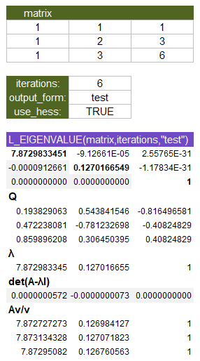
Even with only 6 iterations, using the Hessenberg dramatically improves the convergence. This example is available in the Lambda Library Template which is free to download.
Test: Copy and Paste this LET function into a cell
=LET(
    matrix, {1,1,1;1,2,3;1,3,6},
    iterations, 6,
    output_form, "test",
    use_hess,TRUE,
    EIGENVALUE(matrix,iterations,output_form,use_hess)
)

Result: [see the image below]
=LET(
    matrix,POLYCOMPAN({4,11,-17,-42,0}),
    iterations, 42,
    EIGENVALUE(matrix,iterations)
)

Result:
{  -2.99999999912033,  4.90822979938931,  9.02121195299468,  2.86569861794639;
8.97054354768764E-10,  1.99910252035449,  2.80123179584151,  0.827401461788484;
-1.11397075974907E-27, 0.00120116439609, -1.74910252123416, -0.776222815586076;
                    0,                0,                 0,                  0}
This current eigenvalue function is not ideal for finding the roots of polynomials, but it's working sufficiently for now. Deflation appears to help dramatically with convergence when finding polynomial roots, so that is on the drawing board. Ultimately, a polynomial root finder ought to work with complex numbers, so we have a ways to go yet.
See Also
POLYCOMPAN, QR, HESS
