CSPLINE - Cubic Spline Interpolation
=CSPLINE(known_xs, known_ys, [x], [slopes], [c])
| Argument | Description | Example |
|---|---|---|
| known_xs | The x-values of the control points (column vector) in increasing order | {0;1;2;3} |
| known_ys | The y-values of the control points (column vector) | {4;3;6;1} |
| x | [optional] Values of x to interpolate | {1.5;2.5} |
| slopes | [optional] The slope or tangent at each control point | {0;0} |
| c | [optional, default=0] A value associated with Cardinal splines | 0 |
In the template file, navigate to the Polynomials worksheet to see the CSPLINE function in action.
CSPLINE is used for cubic spline interpolation. It creates a cubic piecewise polynomial that passes through a given set of control points. The derivative of the entire curve is continuous and the slopes at each control point can be specified. The default output is a piecewise polynomial data structure array that can be used by PPVAL for interpolation. If the x parameter is not blank, then the output will be a vector of interpolated values corresponding to the values in x.
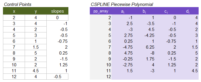 Example control points and resulting cubic piecewise polynomial array
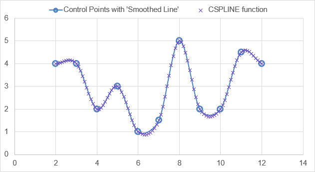 Comparison of CSPLINE with the "Smoothed Line" option in Excel
How it Works
There are many algorithms for different types of cubic splines, so I have provided a detailed explanation of the method used by CSPLINE. It should be noted that this function does not produce a natural cubic spline. Also, the control points must all be unique (no repeated x values) in increasing order. This function does not create loops or circles - only one value of y for each value of x.
Each piece of the Cubic Hermite Spline or "cspline" is a cubic polynomial \(p_i = a_iu^3 + b_iu^2 + c_iu + d_i\) defined by two control points \((x_i,y_i)\) and \((x_{i+1},y_{i+1})\) and the slopes (tangents or first derivatives) at those control points \(m_i\) and \(m_{i+1}\), where \(u_i = (x-x_i)\).
The coefficients for each polynomial can be found by solving a set of 4 linear equations based on the following 4 constraints:
- The curve passes through the first control point \((x_i,y_i)\), or \(p_i(0)=y_i\)
- The curve passes through the second control point \((x_{i+1},y_{i+1})\), or \(p_i(x_{i+1}-x_i)=p_i(u_1)=y_{i+1}\)
- The slope at \((x_i,y_i)\) is \(m_i\), or \(p'_i(0)=m_i\)
- The slope at \((x_{i+1},y_{i+1})\) is \(m_{i+1}\), or \(p'_i(x_{i+1}-x_i)=p'_i(u_1)=m_{i+1}\)
The matrix form of the system of equations \(\bf{A}\bf{x}=\bf{b}\) looks like this:
$$\begin{bmatrix}0 & 0 & 0 & 1 \\ u_1^3 & u_1^2 & u_1 & 1 \\ 0 & 0 & 1 & 0 \\ 3u_1^2 & 2u_1 & 1 & 0 \end{bmatrix}\begin{bmatrix}a_i \\ b_i \\ c_i \\ d_i \end{bmatrix} = \begin{bmatrix}y_i \\ y_{i+1} \\ m_i \\ m_{i+1} \end{bmatrix}$$
We can find the coefficients using \(\bf{A}^{-1}\bf{b}\). However, something really convenient happens if we also scale the interval \([u_0,u_1]\) to \([0,1]\) by dividing \(u\) by \({\Delta}x=(x_{i+1}-x_i)\) and scaling the slopes by multiplying by \({\Delta}x\). That is, the A matrix becomes a matrix of constants with a simple inverse.
$$\begin{bmatrix}0 & 0 & 0 & 1 \\ 1 & 1 & 1 & 1 \\ 0 & 0 & 1 & 0 \\ 3 & 2 & 1 & 0 \end{bmatrix}\begin{bmatrix}a_i({\Delta}x)^3 \\ b_i({\Delta}x)^2 \\ c_i{\Delta}x \\ d_i \end{bmatrix} = \begin{bmatrix}y_i \\ y_{i+1} \\ m_i{\Delta}x \\ m_{i+1}{\Delta}x \end{bmatrix}$$
$$\bf{A}^{-1} = \begin{bmatrix}2 & -2 & 1 & 1 \\ -3 & 3 & -2 & -1 \\ 0 & 0 & 1 & 0 \\ 1 & 0 & 0 & 0 \end{bmatrix}$$
This leads to the following calculations for the coefficients without requiring the algorithm to perform a matrix inversion:
- \(a_i = (2y_i-2y_{i+1}+m_i{\Delta}x+m_{i+1}{\Delta}x)/({\Delta}x)^3\)
- \(b_i = (-3y_i+3y_{i+1}-2m_i{\Delta}x-m_{i+1}{\Delta}x)/({\Delta}x)^2\)
- \(c_i = m_i\)
- \(d_i = y_i\)
Specifying the Slopes
The CSPLINE function allows you to specify the slopes \(m_i\) at each control point. There is also an optional \(c\) parameter that scales each of the slopes as \((1-c)m_i\). The default is c=0. Below are some of the types of cubic Hermite splines that can be created with CSPLINE based on the definitions of \(c\) and \(m_i\).
The input for slopes can be one of 4 options
- {m1,m2,...mn}: Specify all slopes
- m: A single value used for all slopes
- blank: Uses a central finite difference for points 2 through n-1, with forward difference for mstart and backward difference for mend
- {m1,mn}: Specify the starting and ending slopes. Uses a central finite difference for the intermediate points
Forward and Backward Finite Difference
The slope at the first control point, \(m_1\), (if not specified) is calculated using a forward finite difference from the first and second points:
$$m_1 = \frac{y_2-y_1}{x_2-x_1}$$
Likewise, the slope at the last control point, \(m_n\), (if not specified) is calculated using a backward finite difference from the second-to-last and last points:
$$m_n = \frac{y_n-y_{n-1}}{x_n-x_{n-1}}$$
Central Finite Difference
The 3-point central finite difference is used to calculate the slopes at points 2 to n-1. This allows the x values to be non-uniformly spaced. It is equal to the average of the forward and backward finite differences.
$$m_i = \frac{1}{2}\left(\frac{y_{i+1}-y_i}{x_{i+1}-x_i} + \frac{y_i-y_{i-1}}{x_i-x_{i-1}}\right)$$
Cardinal and Catmull-Rom Splines
A Cardinal spline makes use of the additional c parameter which may be in the interval [0,1], and the slopes are calculated using the points before and after the current control point. If the control points are evenly spaced and c=0, the slope is identical to the central finite difference.
$$m_i = (1-c)\frac{y_{i+1}-y_{y-1}}{x_{i+1}-x_{i-1}}$$
When c=1, all the tangents are 0.
A Catmull-Rom spline results when c=0 and the points are evenly spaced. This means that for evenly spaced control points, the default options for CSPLINE result in the Catmull-Rom spline. Due to the default definition for the slopes at the first and last points, there may be some differences between this function and implementations in other software.
The Smoothed Line option in Excel
When you choose the Smoothed Line option in Excel (the blue solid line in the above example), if the x values of the control points are evenly spaced, the smoothed line appears to be a Catmull-Rom spline, but in some cases it is not exactly the same. Therefore, I don't think the algorithm used in Excel is exactly a Catmull-Rom spline.
Lambda Formula
This code for using CSPLINE in Excel is provided under the License as part of the LAMBDA Library, but to use just this function, you may copy the following code directly into your spreadsheet.
Code for AFE Workbook Module (Excel Labs Add-in)
/**
* Cubic Spline - Creates a cubic piecewise interpolating polynomial
* by specifying control points and slopes at each point.
*/
/*
* Inputs:
*   known_xs: A vector of x-coordinates of the control points.
*   known_ys: A vector of y-coordinates of the control points.
*   [x]: (Optional) The x-values at which the spline should be evaluated.
*        If omitted, the function returns the piecewise polynomial data structure.
*   [ms]: (Optional) Slopes at the control points. If omitted, slopes are estimated.
*   [c]: (Optional) Tension parameter for Cardinal splines (default: 0).
*
* Outputs:
*   - Returns either the evaluated spline at x or the piecewise polynomial structure.
*
* Requires: `PPVAL` function to evaluate the piecewise polynomial at x.
*/
CSPLINE = LAMBDA(known_xs, known_ys, [x], [ms], [c],
LET(doc, "https://www.vertex42.com/lambda/cspline.html",
    version, "1.0.0 - Original Version",

    // Step 1: Handle defaults and ensure xs, ys and ms are column vectors
    xs, IF(AND(ROWS(known_xs)=1, COLUMNS(known_xs)>1), TRANSPOSE(known_xs), known_xs),
    ys, IF(AND(ROWS(known_ys)=1, COLUMNS(known_ys)>1), TRANSPOSE(known_ys), known_ys),
    ms, IF(ISBLANK(ms), "", IF(AND(ROWS(ms)=1, COLUMNS(ms)>1), TRANSPOSE(ms), ms)),
    c, IF(ISBLANK(c), 0, c),
    n, ROWS(xs),

    // Step 2: Calculate slopes at each control point
    // Slopes are estimated if not provided explicity
    slope, (1-c) * IF(OR(ms="", ROWS(ms)<=2),
        IF(AND(NOT(ms=""), ROWS(ms)=1),
            SEQUENCE(n,1,ms,0), // All slopes are the same if ms is a scalar
            MAKEARRAY(n,1,LAMBDA(i,j,
                IF(i=1,
                    IF(ROWS(ms)=2,INDEX(ms,1),
                        // Forward difference at the first point
                        (INDEX(ys,i+1)-INDEX(ys,i)) / (INDEX(xs,i+1)-INDEX(xs,i))
                    ),
                    IF(i=n,
                        IF(ROWS(ms)=2,INDEX(ms,2),
                            // Backward difference at the last point
                            (INDEX(ys,i)-INDEX(ys,i-1)) / (INDEX(xs,i)-INDEX(xs,i-1))
                        ),
                        // Central difference at interior points
                        0.5*(
                            (INDEX(ys,i+1)-INDEX(ys,i)) / (INDEX(xs,i+1)-INDEX(xs,i)) +
                            (INDEX(ys,i)-INDEX(ys,i-1)) / (INDEX(xs,i)-INDEX(xs,i-1))
                        )
                    )
                )
            ))
        ),
        ms
    ),

    // Step 3: Compute piecewise polynomial coefficients
    // Each interval [x_i, x_i+1] is represented by a cubic polynomial:
    // P(x) = a*(x - x_i)^3 + b*(x - x_i)^2 + c*(x - x_i) + d
    pp_coeffs, REDUCE(0,SEQUENCE(n-1),LAMBDA(acc,i,
        LET(
            dx,INDEX(xs,i+1)-INDEX(xs,i),
            y_1,INDEX(ys,i),
            y_2,INDEX(ys,i+1),
            m_1,INDEX(slope,i)*dx,
            m_2,INDEX(slope,i+1)*dx,
            coeffs,HSTACK(
                (2*y_1-2*y_2+m_1+m_2)/dx^3,
                (-3*y_1+3*y_2-2*m_1-m_2)/dx^2,
                m_1/dx,
                y_1
            ),
            IF(i=1,coeffs,VSTACK(acc,coeffs))
        )
    )),

    // Step 4: Assemble the piecewise polynomial data structure
    pp,MAP(HSTACK(xs,pp_coeffs),LAMBDA(cell,IFERROR(cell,""))),

    // Step 5: Interpolate if x values are provided, or return coefficients
    IF(ISOMITTED(x),
        pp,
        PPVAL(pp,x)
    )
));
CSPLINE Examples
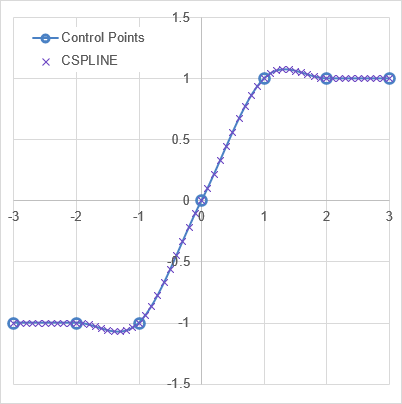
Test: Copy and Paste this LET function into a cell
=LET(
    known_xs, {-3;-2;-1;0;1;2;3},
    known_ys, {-1;-1;-1;0;1;1;1},
    pp_array, CSPLINE(known_xs,known_ys),
    chart_x, LINSPACE(-3,3,61),
    chart_y, PPVAL(pp_array,chart_x),
    HSTACK(chart_x,chart_y)
)

Result: See the image below of the graph of chart_y vs. chart_x
You can interpolate directly with CSPLINE using the optional [x] parameter.
Test: Copy and Paste this LET function into a cell
=LET(
    known_xs, {-3;-2;-1;0;1;2;3},
    known_ys, {-1;-1;-1;0;1;1;1},
    chart_x, LINSPACE(-3,3,61),
    chart_y, CSPLINE(known_xs,known_ys,chart_x),
    HSTACK(chart_x,chart_y)
)

Result: Same result as above.
See Also
NSPLINE, SPLINE, PPDER, PPVAL, PPINT
- Splines in 5 Minutes - YouTube video by professor Steve Seitz
- Wikipedia - Cubic Hermite Spline
- Matlab - spline function (not the same as CSPLINE)
