Newton-Raphson Method in Excel
=SOLVE_NR(function, xstart, [y], [xstep], [epsilon], [iterations], [info])
| Argument | Description | Example |
|---|---|---|
| function | This can be a Named Function or a LAMBDA | myFX |
| xstart | The initial guess at the solution to f(x)=0 | 1 |
| y | Solve for f(x)=y (default is y=0) | 0 |
| xstep | The step size for calculating numerical derivatives (default=0.1) | 0.1 |
| epsilon | The iteration stops when |f(x)|<ε (default=1E-14) | 1E-14 |
| iterations | The maximum iterations allowed (default=20) | 20 |
| info | FALSE (default) returns only final x values, TRUE returns {"x","f(x)","Iteration"}, "verbose" returns every iteration | FALSE |
Newton's Method or the Newton-Raphson Method may be one of the most famous algorithms for solving f(x)=0 for a value of x (also called root-finding for polynomial equations). One of the reasons is its simplicity to both understand and to implement. If a good starting point is chosen, and the function is well behaved, it can also have screaming-fast convergence.
Both Goal Seek and the Excel Solver add-in are powerful optimization tools and solvers for linear and nonlinear equations. Now with the new LAMBDA function, we can also implement Newton's Method using a single Excel formula.
SOLVE_NR is essentially a version of Goal Seek (which uses the Newton-Raphson method) that can be used to solve an equation that you define as a LAMBDA. Your LAMBDA function needs to accept a single value (x) as an input like LAMBDA(x, expression).
The Bad News : SOLVE_NR cannot iteratively change other input cells within your spreadsheet. So, even though the algorithm is similar to that used in Goal Seek,
Table of Contents
Building the Newton-Raphson Function
To both explain how the Newton method works and also show how it works specifically with Excel, I'll explain how to build this Newton-Raphson LAMBDA function from scratch. We're not going to embelish the algorithm with anything fancy. Just bare-bones Newton-Raphson.
Step 1: Define the Function f(x)
For the sake of demonstration, we'll define our function as f(x)=SIN(RADIANS(x))+x/360 and give it the name myFX(x). If we were going to use this function throughout the worksheet, we could use the Name Manager, but for the sake of this demonstration, we'll do everything within LET, so you can copy and paste this LET function into Excel. If you are using a recent version of Excel, it should work for you.
=LET(myFX,LAMBDA(x, SIN(RADIANS(x))+x/360 ),
    myFX(10)
)

Result: 0.201425955 ... just a quick test to see that myFX is working.
Step 2: Graph the Function
When using Newton's method, it's always a good idea to graph your function if possible. To do this, we just need a range of x values and then we'll calculate myFX(x) for each of these values. Given the nature of our function, we can give it an array of x values and it will return the corresponding y values. But, if your function is not vectorized, you can use BYROW like this:
=LET(myFX,LAMBDA(x,SIN(RADIANS(x))+x/360),
    x_values, LINSPACE(-720,720,2001),
    y_values, BYROW( x_values, LAMBDA( value, myFX(value) ) ),
    VSTACK({"X","Y"},HSTACK(x_values,y_values))
)
After you have your X and Y values in Excel, you can plot it using a simple XY Scatter chart.
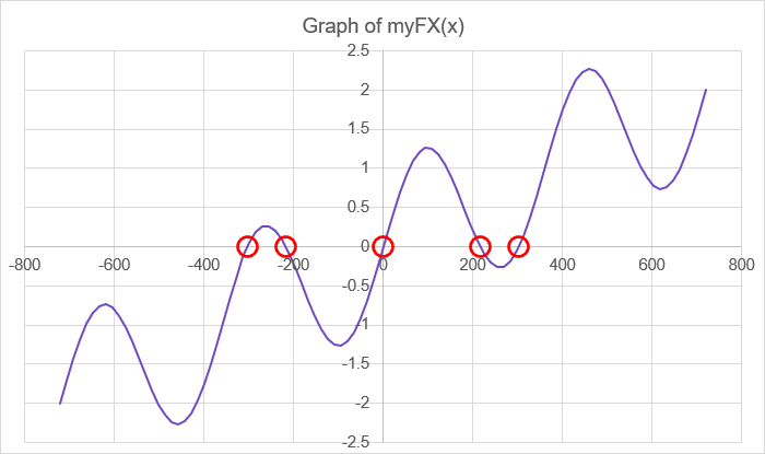
You can see from the graph of this function, that it has five possible solutions for f(x)=0 somewhere between [-400,400] (circled in red). One is obvious (x=0), but we'll use Newton's Method to find the others.
Step 3: Start With a Guess, x0
Although technically we are on step 3, the first two steps were just us getting ready to implement Newton's Method. That's where we are at right now. Our "first step" is to start with a guess for x where f(x) is 0.
If you have graphed the function already, then you pick a rough value for where the function crosses the x-axis. From a visual inspection, I'd probably start with x=-300, x=-200, x=200, or x=300.
The xstart parameter for our function is this initial guess x0=200. We also want to evaluate f(x0) to see how close to zero we are with our first guess. Remember that in Excel you can't use parameter names that are cell references, so x0, x1, f0, f1 are off limits as variable names. Our updated formula:
=LET(myFX,LAMBDA(x,SIN(RADIANS(x))+x/360),
    xstart, 200,
    f_xstart, myFX(xstart),
    output,VSTACK({"x","f(x)","Iteration"},HSTACK(xstart,f_xstart,0)),
    output
)

Result:
{          "x",         "f(x)",  "Iteration";
           200,      0.2135354,            0}
Step 4: Find the Derivative, f'(xn)
The Newton-Raphson Method relies on the derivative of the function, f'(x) often referred to as "f prime." In numerical methods, we typically use finite difference to calculate the derivative.
Choose a Step Size: Based on the x-axis scale and the fact that our function is continuous, we'll use a value of 0.01 for the xstep parameter. Note that in our example, the units for x is degrees. Stepping a small 0.01 degree is going to give us a decent estimate of the derivative at x.
The numerical derivative, using a forward difference, is (f(xn+∆x)-f(xn))/∆x where ∆x=xstep. This involves calling our predefined function myFX(x) two times:
fprime_xstart = (myFX(xstart+xstep)-myFX(xstart))/xstep
Step 5: Step Closer to Zero
Using Newton's Method, we can find a new (hopefully better) guess for f(x)=0 using xn+1=xn-f(xn)/f'(xn). For now, xn is xstart and xn+1 will be xnew. We'll then calculate the new value for f(xn+1) as fnew = myFX(xnew).
We have now completed the first iterations of Newton's Method, and here is our updated Excel formula:
=LET(myFX,LAMBDA(x,SIN(RADIANS(x))+x/360),
    xstart, 200,
    f_xstart, myFX(xstart),
    xstep, 0.01,
    fprime_xstart, (myFX(xstart+xstep)-myFX(xstart))/xstep,
    xnew, xstart - f_xstart/fprime_xstart,
    fnew, myFX(xnew),
    output, VSTACK({"x","f(x)","Iteration"},
                   HSTACK(xstart,f_xstart,0),
                   HSTACK(xnew,fnew,1)),
    output
)

Result:
{          "x",         "f(x)",  "Iteration";
           200,      0.2135354,            0;
    215.675279,      0.0159072,            1 }
Step 6: Iterate Until f(x) is Very Small
We now just need to repeat steps 5 and 6 until f(xnew) is very small or until we reach our iteration limit. It is useful to see how the values change as the algorithm proceeds, so we'll want to continue having the option to output the results of each iteration.
If creating a loop in an Excel formula is new to you, I'd encourage you to review the Create LAMBDA Functions article, especially the discussion of recursion and the REDUCE function.
Here is the same formula from step 5 rewritten with a loop. Notice that iterations=1 will yield the same result as step 5.
=LET(solve_for, 0,
    myFX, LAMBDA(x, SIN(RADIANS(x))+x/360 - solve_for),
    xstart, 200,
    f_xstart, myFX(xstart),
    xstep, 0.01,
    iterations, 1,
    initial, VSTACK({"x", "f(x)", "Iteration"}, HSTACK(xstart, f_xstart, 0)),
    loop, REDUCE( initial, SEQUENCE(iterations), LAMBDA(acc, i,
        LET(
            row, TAKE(acc, -1),
            xn, INDEX(row, 1, 1),
            fn, INDEX(row, 1, 2),
            fprime, (myFX(xn + xstep) - fn) / xstep,
            xnew, xn - fn / fprime,
            fnew, myFX(xnew),
            output, VSTACK(acc, HSTACK(xnew, fnew, i)),
            output
        )
    )),
    loop
)
To continue building up our output, we use the REDUCE function with an incrementer i to represent our iteration and an accumulator (acc) that stores the entire output array. Notice that we've initialized the accumulator with the array initial which consists of the same output that we created in Step 3.
At each iteration within the REDUCE "loop" we do the following:
- Get the last row from the accumulator using TAKE
- Get xn and fn from that row using INDEX
- Calculate fprime using one additional call to myFX
- Calculate xnew then fnew using another call to myFX
- Stack our new results onto the end of the accumulator
Let's try iterations=5:
{            "x",             "f(x)", "Iteration";
200             ,  0.213535412229887,           0;
215.675278952046,  0.015907224586377,           1;
217.070740325279,  0.000173677870134,           2;
217.086320806385,  0.000000007984292,           3;
217.086321522833, -0.000000000000658,           4;
217.086321522774,       2.220446E-16,           5}

SOLUTION: x=217.086321523
2.220446E-16 is probably close enough to zero for our purposes, so we have our first solution (second, if you count already knowing that x=0 is a solution).
Notice how quickly f(x) approaches zero? You can almost see (from the shape of the red numbers) how this algorithm has quadratic convergence.
SOLVE_NR - Taking it a Step Further
The SOLVE_NR function in this LAMBDA Library below takes things a bit further than what we did above, but it's still basically the same function as the one we just assembled. Here are the other things I've added:
- Multiple start values: You can specify xstart as an nx1 vector of start values. The function will run the algorithm for each value in turn (like running Goal Seek for multiple start values).
- Multiple output options: The info parameter can be FALSE (default) to return only the final x value(s), TRUE for a bit more information, or "verbose" to show the results of all the iterations. See the example below.
- Control over iterations and precision: The function lets you have some control over the precision of the final result (by specifying a value for epsilon) and the number of iterations.
- Solve for f(x)=y: Like Goal Seek, you can choose to solve for a specific value of y (the default is y=0).
How Does This Compare to Goal Seek?
Try It! In cell B1, enter =SIN(RADIANS(A1))+A1/360. Enter 500 into cell A1. Run Goal Seek (Data > What-If) telling it to set B1 to 0 by changing A1. Does it converge?
Next, set A1 to 200 and run Goal Seek again. What is the result? I got A1=217.085 with B1=1.44E-5. This isn't as precise as our homemade Newton's Method above!
So, does SOLVE_NR beat Goal Seek? Not necessarily.
The biggest limitation of SOLVE_NR is it cannot change the values of other cells like Goal Seek or Solver. With enough time and effort, many complex spreadsheet models can be turned into a lambda function, but for a quick analysis, Goal Seek, Solver, or Data Tables may be easier and faster.
One benefit of SOLVE_NR is the ability to recalculate automatically whenever you change other inputs in Excel (unlike Goal Seek which you have to manually run each time).
Also, you can use SOLVE_NR within your model and even run Solver and Goal Seek (or Data Tables) with SOLVE_NR as part of your model: a solver within a solver.
As an educational tool, the SOLVE_NR function allows you to set the info parameter to "verbose" to see the results of every iteration (see the example below).
Why is the Number of Function Calls Important?
Algorithms like this that rely on iteration and recursion make repeated calls to what might be a very complex function. Imagine if your model took 10 seconds to finish a single evaluation. In the above example, we called the myFX function 1+2*5=11 times. If each call was 10 seconds, then this would have taken almost 2 minutes to complete.
The reality is that Excel will essentially just "hang" if a function takes that long. But in the world of solver algorithms, convergence rate and the number of function calls is a big deal as the models become more complex and therefore take longer to evaluate.
What if I Want to Solve for f(x)=5?
Not a problem. Just change your function to g(x)=f(x)-5 and solve for g(x)=0.
One of the reasons why this algorithm and others are designed to solve for f(x)=0 is that if f(xn) becomes negative at some point in the iteration, the search direction automatically takes the reverse sign, which drives it back to zero.
The SOLVE_NR function includes solving for f(x)=y as an option.
Make it Stop!
Rather than continue iterating until the maximum iterations has been reached, the SOLVE_NR function will stop iterating when the value for |f(xn)| is less than ε=1E-14. If you want to change that level of precision, you can specify a different value for epsilon (within the limits of Excel's precision).
Although REDUCE will cycle through the entire number of iterations specified (or 20 by default), after it hits the ε precision goal, it just quickly skips through the rest of the iterations by returning acc instead of proceeding with the other calculations.
Note that the precision is based on the value of f(x) being close to zero, not the change in x.
Failure to Converge?
There is still a need for specifying the number of iterations, because Newton's Method is notorious for failing to converge. In fact, a good example of that is to start the function from Step 6 at xstart=500. Set the iterations to 20 and see what happens.
The tangent (derivative) at x=500 points down to the x-axis to about x=700 (691.8 according to iteration #1). And then it just sort of sits there and oscillates, never able to get back over into the x=300 range.
A poor start combined with highly nonlinear = poor convergence for Newton-Raphson.
Some possible reasons for not converging are:
- Derivative is Zero: If it wanders into a flat region or evaluates the derivative to be zero, you'll have a 1/0 error.
- Iteration enters a Cycle: Like our example above starting at 500.
- Function is undefined or errors: The function cannot be evaluated at the value for x for some reason, either mathematically or due to calculation errors.
- Discontinuous derivative: If the derivative is not continuous near the root, it can get thrown off and never converge at the root.
SOLVE_NR Lambda Formula
This code for using SOLVE_NR in Excel is provided under the License as part of the LAMBDA Library, but to use just this function, you may copy the following code directly into your spreadsheet.
Code for AFE Workbook Module (Excel Labs Add-in)
In anticipation of this function possibly changing (improving) over time, it includes the version number.
/**
* Newton-Raphson Method equation solver for finding f(x)=0
*/
SOLVE_NR = LAMBDA(function,xstart,[y],[xstep],[epsilon],[iterations],[info],
LET(doc,"https://www.vertex42.com/lambda/newton-raphson.html",
    version,"1.0.0",
    n,ROWS(xstart),
    y,IF(ISOMITTED(y),0,y),
    xstep,IF(ISOMITTED(xstep),0.1,xstep),
    epsilon,IF(ISOMITTED(epsilon),1E-14,epsilon),
    iterations,IF(ISOMITTED(iterations),20,iterations),
    ret,REDUCE({"x","Fx","Iterations"},SEQUENCE(n),LAMBDA(acc_row,i,
        VSTACK(acc_row,
        REDUCE(
            HSTACK(INDEX(xstart,i),function(INDEX(xstart,i))-y,0),
            SEQUENCE(iterations),
            LAMBDA(acc,k,
            LET(cur_row,TAKE(acc,-1),
                IF(ABS(INDEX(cur_row,1,2))<ABS(epsilon),acc,
                    LET(
                        xn,INDEX(cur_row,1,1),
                        fn,INDEX(cur_row,1,2),
                        fprimen,(function(xn+xstep)-y-fn)/xstep,
                        xnew,xn-fn/fprimen,
                        fnew,function(xnew)-y,
                        new_row,HSTACK(xnew,fnew,k),
                        output,IF(info="verbose",VSTACK(acc,new_row),new_row),
                        output
                    )
                )
            ))
        ))
    )),
    IF(OR(info=TRUE,info="verbose"),ret,DROP(ret,1,-2))
));
Named Function for Google Sheets
Name: SOLVE_NR
Description: SOLVE_NR Function for Newton-Raphson in Excel
Arguments: function, xstart, xstep, epsilon, epsilon
Function:

[Still in the works]
Version 1.0.0: Published 2/8/2024 by Jon Wittwer
SOLVE_NR Examples
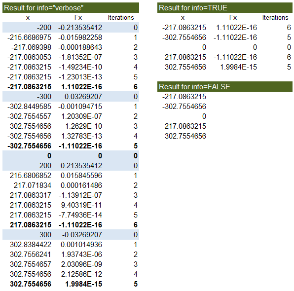
Test: Copy and Paste this LET function into a cell
=LET(
    myFX, LAMBDA(x, SIN(RADIANS(x))+x/360),
    xstart, {-200;-300;0;200;300},
    info, "verbose",
    SOLVE_NR(myFX,xstart,,,,info)
)
Result: (see below)
Find a set of starting guesses for the roots of a 6th degree polynomial and then use SOLVE_NR to find the roots. Even though we've graphed the polynomial and could just look at the graph to come up with 6 values for xstart, we'll use a different approach.
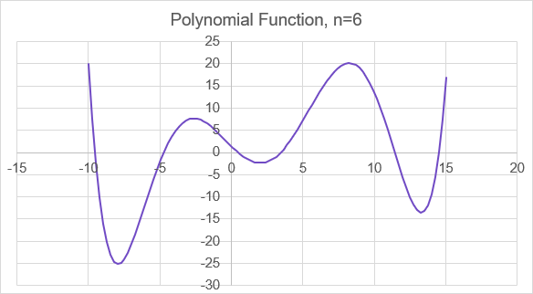
We are creating an x vector between [-10,15] with 1001 points and then evaluating the polynomial for all of those values, looking for sign changes. Those sign changes are locations where the function crosses the x-axis and therefore are decent starting points for SOLVE_NR.
The LAMBDA function in red below takes the place of defining a custom named function such as myFX in our example above. The graph above is a graph of pxvec vs. xvec.
Test: Copy and Paste this LET function into a cell
=LET(
    px_coeffs, {0.0001164,-0.001812,-0.01309,0.21,0.2985,-3.195,1.403},
    steps, 1001,
    xvec, LINSPACE(-10,15,steps),
    pxvec, POLYVAL(px_coeffs,xvec),
    signchange,VSTACK(FALSE,SIGN(DROP(pxvec,1,0))<>SIGN(DROP(pxvec,-1,0))),
    xstart,INDEX(xvec,FILTER(SEQUENCE(steps),signchange)),
    solutions,SOLVE_NR( LAMBDA(x,POLYVAL(px_coeffs,x)), xstart,0,0.0001,1E-8,,TRUE),
    solutions
)

Result: xstart = {-9.55;-4.7253;0.475;3.45;11.45;14.525}

Result: solutions =
{       "x",               "Fx",        "Iterations";
 -9.56107456809315, 2.09032791076424E-12,     3;
 -4.73162758403092, 1.47077328094269E-09,     2;
  0.46583704630151,-8.32470981038114E-10,     2;
  3.44611343423515, 5.38752598089332E-10,     2;
  11.4396751791338,-1.28785870856518E-14,     2;
  14.5080868023951, 3.79940523487221E-11,     3}
This brute-force method of finding the locations of the sign changes is not something you'd want to do by hand (or with a function that takes a long time to evaluate), but with a small enough step size and fast enough function, it can be a decent method for finding real roots of a polynomial between [xmin,xmax]. But, here we are just using the technique to find starting values for our Newton-Raphson solver.
