One of the best ways to learn new techniques in Excel is to see them in action. This post demonstrates how to add some fun and useful features to simple to do lists including drop-down lists, check boxes, progress bars, and more. The images show Excel 2016, but instructions are similar for Excel 2010 and Excel 2013.
This Page (contents):
- Simple Drop-Down Lists via Data Validation
- Conditional Formats for the Priority Column
- Conditional Formats for Numeric Priority
- Checkboxes using Form Fields
- Checkboxes via Data Validation
- Progress Bar for % Completed
- Gray-Out Tasks When They are Complete
- Highlighting Overdue Dates
- Autofilter and Sorting
- Create a Gantt Chart
- Drop-Down with Current Date
1. Simple Drop-Down Lists via Data Validation
Many task lists include a Priority or Status column, such as the Homework To Do List shown below. It's very handy to use an Excel drop down list for columns like these.
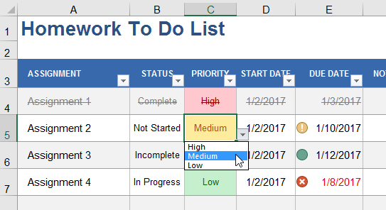
To create a simple drop-down list, follow these steps:
- Select the cells you want to edit
- Go to Data > Data Validation
- Choose "List" in the Allow field
- In the Source field enter a comma-delimited list such as High,Medium,Low
2. Conditional Formats for the Priority Column
In the example above you will see that the values in the Priority column have been highlighted differently. This can be done automatically and is a great way to easily identify your high-priority tasks. Follow these steps to create the type of formats shown in the example above.
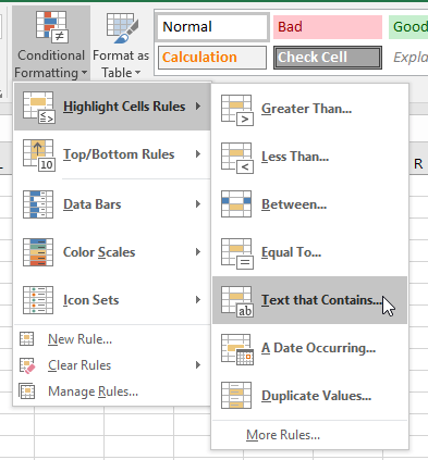
- Select the cells in the Priority column
- Go to Home > Conditional Formatting > Text That Contains
- Enter the word high and choose the "Light Red Fill with Dark Red Text" option
The image below shows how to get to the correct option from the Home tab.
3. Conditional Formats for Numeric Priority
If you want to use a numeric priority like 0-4, then you can use Icon Sets to display images instead of (or in addition to) the numeric value. You can see this demonstrated in the Simple Task Tracker below.
![]()
- Select the cells in the Priority column
- Create a drop-down list with the options 4,3,2,1
- Go to Home > Conditional Formatting > Icon Sets > More Rules
- The image below shows you how to modify the settings for this rule.
![]()
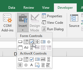
4. Checkboxes using Form Fields
I don't like this method. If you like to sort and delete and insert rows, form fields get all messed up. They may be nice for a spreadsheet layout that is not meant to be modified, but so far I haven't found a to do list that I haven't wanted to modify frequently.
The form field checkbox is found in the Developer tab shown in the image below. If you don't see the Developer tab, go to File > Excel Options > Customize Ribbon and find and check the Developer tab.
5. Checkboxes via Data Validation
I wish Microsoft would add an in-cell checkbox feature (Apple's Numbers software does it), but until they do that we have to come up with clever alternatives.
One method I like is using a data validation drop-down list because it works pretty well in Excel on touch-enabled devices, and it is also compatible with most versions of Excel and OpenOffice and Google Sheets.
The simplest checkbox to make using a drop-down list is probably just a list with a single character (x), or you could use a special character like the square root sign (√) that looks like a check mark in some fonts. In the example below, I've used this technique plus a small square ascii character (□,√).
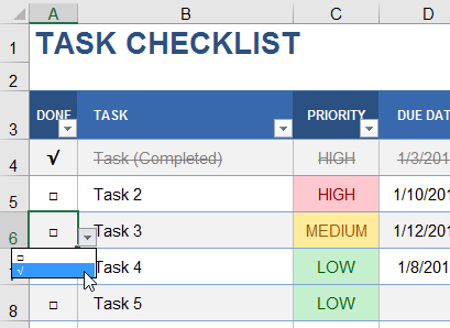
Another approach that I really like is to use custom Icon Sets via Conditional Formatting. This isn't as compatible with other spreadsheet programs (like Google Sheets) but it looks good. The simple Task Tracker Template shows an example of this:
![]()
- Select the cells you want to use for the check boxes
- Create a drop-down list with the options 1,0,-1
- Go to Home > Conditional Formatting > Icon Sets and select any set you like
- With those cells still selected, go to Home > Conditional Formatting > Manage Rules and find the rule you just created and edit it to create a custom icon set with the setting shown in the following image.
![]()
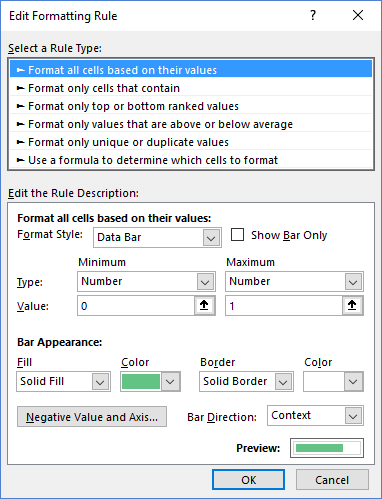
6. Progress Bar for % Completed
In some of the examples above, you've already seen progress bars in the "% Complete" column. Now you'll learn how to do it. Conditional formatting comes in handy yet again:
- Select the cells in the % Complete column
- Go to Home > Conditional Formatting > Data Bars > More Rules
- Modify the bar based on the settings shown in the image below
Want a Progress Bar in Google Sheets? No problem. In cell A1 enter the % Complete and then in the cell to the right of it you can use the formula =REPT("█",ROUND(A1*10,0)). You can change the color of the bar by just changing the font color. That's a pretty old trick for Excel users, but it's something that will work in Google Sheets, too.
Progress Bar via SPARKLINE in Google Sheets
The new SPARKLINE function allows you to create a progress bar in Google Sheets very easily. Enter a percent complete in cell A1 and the following SPARKLINE function for the bar chart in cell A2.
A1=87.2%
A2=SPARKLINE(A1,{"charttype","bar";"color1","blue";"max",1;"min",0})
See the Simple Gantt Chart (Google Sheets version) for an example of how the SPARKLINE function can be used for progress bars.
For more ways to modify the color and look of the in-cell progress bar, see the SPARKLINE function documentation.
7. Gray-Out Tasks When They are Complete
If you like the effect of seeing your completed tasks crossed out or grayed out or both, you can do that fairly easily using conditional formatting.
In the example below, the first rule is applied when column A is equal to the special square root character. The placement of the dollar sign in the $A4 reference is very important in this formula because we want all the columns in the table to reference column A.
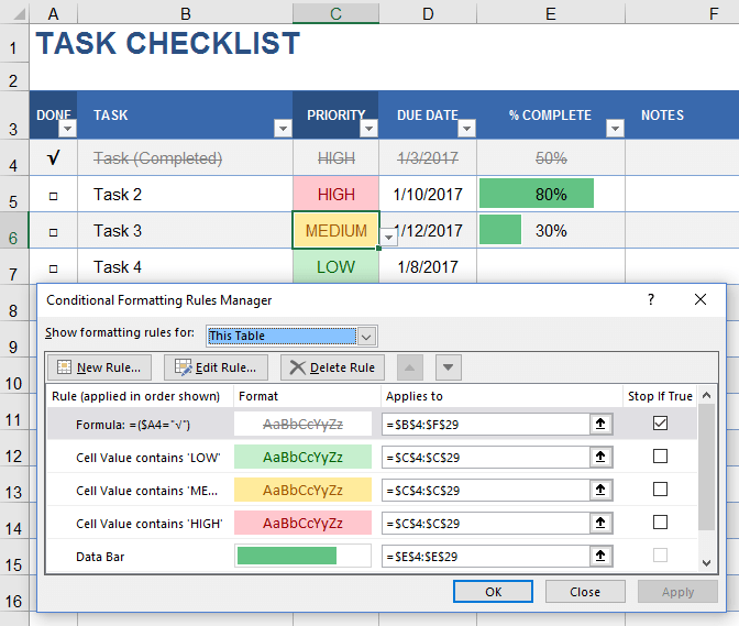
Also note that the first rule has the "Stop if True" box checked. That is why you don't see the priority cell highlighted red or the % Complete showing a green bar in the example. When the task is marked as complete, I don't want to be distracted by formatting that no longer matters to me. So I'm using the rule order to prevent the following rules from being applied if the task has been marked as done.
8. Highlighting Overdue Dates
When you have a Due Date, you may want to highlight the date when it is overdue. You can do that with a simple conditional formatting rule shown in the example below.
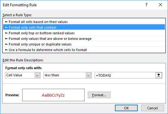
You can see an example of this in the Homework To Do List shown at the very top of this article.
9. Autofilter and Sorting
The little arrows that show up in the header of an Excel table or list are a result of turning on the Filter Button feature. If you don't see the little arrows in the header row already, select a cell in your table (or the entire table) and go to the Data tab and click on the Filter button.
10. Create a Gantt Chart
Although a Gantt chart is a great visualization and management tool for projects, creating one from scratch is not nearly as simple as the other ideas shared in this article. The two most common ways to create a Gantt chart in Excel are (1) using a stacked bar graph chart object and (2) using conditional formatting. Visit my Task List Templates page to find an example that uses a chart object and try the free Gantt Chart Template to see the conditional formatting technique in action.
11. Drop-Down with Current Date
Update 10/9/2018 - I recently created a new wedding checklist where a user requested the ability to enter either a checkmark or the current date. To do this with data validation, create a list somewhere in the worksheet with the first cell containing a check mark unicode character ✔ and the next cell containing the formula =TODAY().
Then, use data validation to create a drop-down list referencing those two cells. This will allow you to select either a checkmark or the current date as shown in the image below.
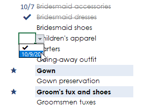
To avoid having Excel show warnings when cells contain older dates, make sure to turn off the warnings and errors when setting up the data validation.


Comments
I really like these ideas. The method for adding a progress bar in Google Sheets is a great work-around.
Hello,
great post, this is actually basic but you just have explained in a better way.
i enjoyed reading.
keep sharing
These are excellent features. I’m looking for a way to have a tab for each one of my projects (lets say 10 projects – each have a tab) and then for them to be summarized by person and/or project on a “summary” tab. Is this possible in Excel?
@Good … Yes, that should be possible. Might not be easy to create the summary tab, but you might as well give it a try.
Hi,
Thank you for all of your great templates.
These templates say they are only for iPad/iPhone? Not for desktop?
https://www.vertex42.com/ExcelTemplates/task-list-template.html
Thank you,
best regards, Marjolein
@Marjolein, you may have missed the AND sign, meaning AND Excel for iPad/iPhone.
Is it possible to have completed tasks automatically move from a “Pending” tab to a “Completed” tab?
@Elizabeth, Possible yes, but not without VBA macros. If you make a copy of the worksheet, you can label one as “Completed” and use cut/paste to move rows from one worksheet to the other.
Hi! Is it possible to add automatically add a “Done Date” when changing the status to Complete? Thanks :)
Great tips, btw! Very helpful!
@Patricia. You would need to create a new column for storing the date. You’d have to add some custom VBA code if you wanted the date to be entered automatically when changing Done to 100%. Or, you can press Ctrl+; to enter the current date.
in excel on your Project Task List Template is there any way after you sort to always keep the PROJECT TITLE visible. please help thank you Rob
You could use Freeze Panes to keep the upper rows visible as you scroll.
Didn’t you attached the template?
Hi, John!
Great products! Does the Gantt Chart Pro have the priority task option with drop-down? If not, is there a way to add the feature? We need the feature to work with google sheets for our team.
HI
How to add more projects to list please?
I am creating a worksheet of many categories of my work and would like the most priority ones show up on the front tab. Do you know how would I go about to achieve this?
Also, any app like monday.com or airtable you would recommend using as well?
@Eva … In Excel, assembling a separate filtered list from a different table is usually done with a Pivot Table.
Spreadsheet.com is still under development, but I’m excited about how it’s turning out. Airtable does a lot of great things as a simple-to-use database program, but when spreadsheet.com finishes the development of the built-in gantt chart and calendar tools, it’s going to be a very competitive project management app.
Very well explained. Thanks for the much needed info.