In Excel, a dynamic range is a reference (or a formula you use to create a reference) that may change based on user input or the results of another cell or function. It is more than just a fixed group of cells like $A1:$A100. I use dynamic ranges mostly for customizable drop-down lists. To avoid showing a bunch of blanks in the list, I use a formula to reference a range that extends to the last value in a column. The image below shows 4 different formulas that reference the range A2:A9 and can expand to include more rows if the user adds more categories to the list.
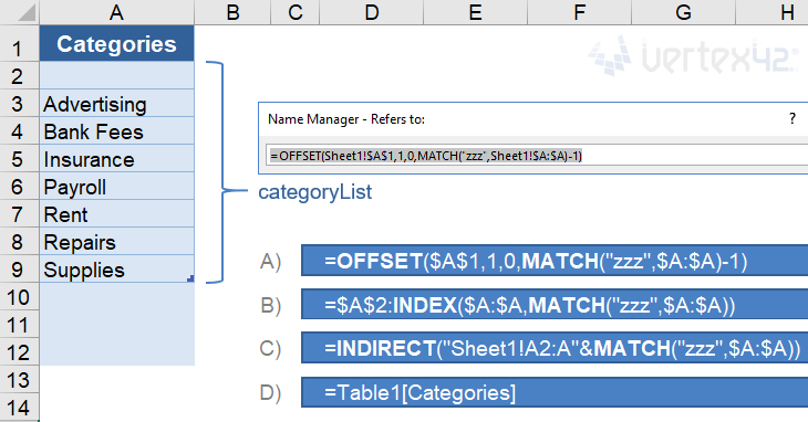
When we talk about a dynamic named range, we're talking about using the Name Manager (via the Formula tab) to define a name for the formula, such as categoryList. We can then use that Name in other formulas or as the Source for drop-down lists.
This article isn't about the awesome advantages of using Excel Names, though there are many. Instead, it is about the many different formulas you can use to create the dynamic named ranges.
To see these examples in action, download the Excel file below.
Download the Example File (DynamicRanges.xlsx)
Do you have a Dynamic Named Range challenge you need to solve? If you can't figure it out after reading this article, go ahead and ask your question by commenting below.
This Page (contents):
- A) The OFFSET Function
- B) The INDEX Function for a Non-Volatile Dynamic Range
- C) The INDIRECT Function
- D) Structured References with Excel Tables
- E) The CHOOSE and IF Functions
- Find the Position of the LAST Value in the Column
- Bonus: Create a Dynamic Print Area
- No Dynamic Named Ranges in Google Sheets
Watch the Video
A) The OFFSET Function
The most common function used to create a dynamic named range is probably the OFFSET function. It allows you to define a range with a specific number of rows and columns, starting from a reference cell. The syntax for the OFFSET function is:
=OFFSET(reference,offset_rows,offset_cols,[height],[width])
The offset_rows and offset_cols values tell the function where you want the upper-left cell of your range to be, relative to the reference cell. The height and width values tell the function how many rows and columns you want to include in your range.
A Basic Customizable List
In the meal planner template, I have a list of meals that I use as the Source for many different drop-down lists. I want to allow the user to edit and add to the list, so the dynamic named range used by the drop-down needs to extend to the last value in the list. I could define the range as $A:$A (the entire column) or $A1:$A1000 (assuming they won't add more than 1000 items to the list), but then I'd end up with a bunch of blank cells at the end of my drop-down list.
Using the OFFSET function, I define a range that starts at cell $A$1 and ends at the cell containing the last value in the column. If the last value in the column was on row 15, the formula for the named range would be:
=OFFSET($A$1,0,0,15,1)
To make this formula dynamic, I'll use a formula or reference in place of the height value (15) to specify how many rows I want the range to include. I expect only text values in this list, so I'll use the MATCH function to find the last text value in the column like this:
=OFFSET($A$1,0,0,MATCH("zzzz",$A:$A),1)
There are many formulas you can use to determine the height or width of the range, such as COUNTA, COUNT, VLOOKUP, LOOKUP, MATCH or various array formulas. What formula you use may depend on whether you expect there to be blank cells in the list, error values (like #N/A or #DIV/0!), or data of different types (text or numeric or both), and whether calculation speed is an issue.
Later in this article I'll talk more about the various formulas for finding the last value in the range. For now, we'll continue using MATCH.
A Robust Dynamic Range
When you allow a user to edit a list, they may end up deleting the first row in the list, or they might insert a row above the first row in the list (between the label row and the first item). To create a formula that works in spite of these actions by the user, I like to use a label for the reference and include the label in the range, as shown in the following examples.
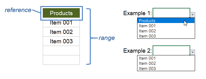
Example 1: Include the label in the list
=OFFSET(reference,0,0,MATCH("zzz",range),1)
Example 2: Exclude the label from the list
=OFFSET(reference,1,0,MATCH("zzz",range)-1,1)
Notice in the second example that reference and range have not changed. To exclude the label from the list, we are using an offset of 1 row and subtracting one row from the number returned by the MATCH function.
B) The INDEX Function for a Non-Volatile Dynamic Range
A volatile function within a cell or named range is recalculated every time any cell in the worksheet recalculates (instead of just when one of the function's arguments changes). Also, any formula that depends on a cell containing a volatile function is also recalculated. If you have a large file with thousands of inefficient formulas that reference a cell containing a volatile function, Excel may seem to take forever to recalculate. OFFSET is a volatile function. INDEX is not, so some people prefer to use INDEX for dynamic ranges.
The INDEX function can return the reference to a range or cell instead of just the value. That means that just like OFFSET, you can use INDEX in many places where Excel is expecting a cell reference. For example, to create the range A1:A4 you can use INDEX(A:A,1):INDEX(A:A,4).
We can use INDEX to create the same dynamic ranges shown in the OFFSET examples:
Example 1: Include the label in the list
=INDEX(range,1):INDEX(range,MATCH("zzz",range))
Example 2: Exclude the label from the list
=INDEX(range,2):INDEX(range,MATCH("zzz",range))
To exclude the label (the first cell in the range), the only change we needed to make was the "2" in INDEX(range,2). Using INDEX(range,1) and INDEX(range,2) instead of just a cell reference makes the formula more robust. It prevents the problem of having the reference changed to #REF! if the reference row gets deleted.
NOTEWhen using INDEX, the formulas cannot be entered directly as the Source for a drop-down list. But, if you create the formula as a dynamic named range, you can use the name as the Source for the drop-down list.
By the way, I learned about using the INDEX function to make a non-volatile dynamic range from Mynda Treacy at MyOnlineTrainingHub.com and Debra Dalgleish at Contextures.com.
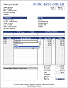 Purchase Order with Price List
See Dynamic Named Ranges in action. This template uses multiple customizable lists for selecting items descriptions, vendor and ship to addresses, and other options. The item description list uses the OFFSET formula and the other lists use the INDEX formula.
C) The INDIRECT Function
The INDIRECT function is another awesome function for creating dynamic ranges. It is also a volatile function, but like I mentioned above, that might not matter. The INDIRECT function lets you define a reference from a text string, and you can use concatenation to create the text string, like this:
=INDIRECT("Sheet1!A1:A"&row_num)
In the example shown at the top of this post, to create the reference "Sheet1!A2:A9" we replace row_num with MATCH("zzz",$A:$A) to return the row number of the last text value.
Important: When using INDIRECT to reference a range on a different worksheet, don't forget to include the worksheet name in the string. When you enter a reference in the Refers To field via the Name Manager, Excel will automatically change $A:$A to "Sheet1!$A:$A" but it won't know how to change your text string. This is one of the cons to using INDIRECT because if you change the name of the worksheet, you'll need to remember to update your INDIRECT formula.
D) Structured References with Excel Tables
Beginning with Excel 2007, Microsoft introduced a new way to work with data in what are called Excel Tables, not to be confused with Data Tables, or other generic uses of the term table (yes, it is confusing).
If you use an official "Excel Table," you can use a type of reference known as a structured reference. The structured reference uses the table name and the column labels like this:
=Table1[Categories]
You don't need to know how to type the correct structured reference. While you are entering a formula, if you select the column in the Table, Excel will automatically change your reference to the structured reference.
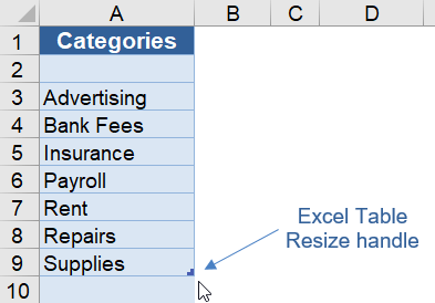
The reason these types of references can be considered dynamic is because of the unique way that table references behave when you expand or contract the table. Meaning, if you extend the table down by dragging the resize handle in the lower-right corner of the table, the reference =Table1[Categories] will automatically include the new rows.
So, instead of using an OFFSET formula to extend a range to the last value in a customizable list, we can let the user change the size of the list using the drag handle. Of course, this requires the user to know how to use Tables and the drag handle. That is one of the reasons I don't often use this technique in my templates (that, and lack of compatibility with OpenOffice and Google Sheets).
E) The CHOOSE and IF Functions
Although I don't use the CHOOSE function or nested IF formulas to create lists of variable length, they are pretty powerful functions for creating other types of dynamic ranges. For example, the two formulas below both return a different range (range_1, range_2 or range_3) based on a given number:
=CHOOSE(number,range_1,range_2,range_3,...)
=IF(number=1,range_1,IF(number=2,range_2,IF(number=3,range_3)))
The CHOOSE function is basically a shortcut for the nested IF formula in this case. When possible, I prefer using CHOOSE over nested IF formulas (if only to avoid having a million closing parentheses at the end of the formula ))))))))))).
See CHOOSE in action: My article "Create a Drop Down List in Excel" shows an example using CHOOSE to create a dependent drop down list.
Find the Position of the LAST Value in the Column
When using a dynamic named range for lists of variable length, we need to know how to find the numeric position of the last value in the column. In the examples above we used MATCH("zzz",range) for text values, but for numeric data or a combination of text and numeric data we may need to use something different. The formulas below cover all the scenarios I've come across.
The following image will be used for the example. It shows the reference and range and the position numbers of the values in the range.

1. Find the Position of the Last Numeric Value
The following formulas will allow the range to include blanks, error values, and text values, but the formulas will only return the position of the last numeric value. The result would be 4 in the example above.
=MATCH(1E+100,range,1)
=LOOKUP(42,1/ISNUMBER(range),ROW(range)-ROW(reference)+1)
See my article about VLOOKUP and INDEX-MATCH for a more detailed explanation of these MATCH and LOOKUP formulas. LOOKUP does not behave the same way in OpenOffice and Google Sheets. So, for maximum compatibility, I still prefer to use MATCH.
The value 9.99999999999999E+307 could be used for the MATCH function because it is the largest numeric value that can be stored in a cell, but that is kind of overkill. I prefer to use something more concise like 1E+100 or 10^100 (a googol).
2. Find the Position of the Last Text Value
The following formulas will allow the range to include blanks, error values, and numeric values, but the formulas will only return the position of the last text value (row 5 in the example above).
=MATCH("zzzz",range,1)
=LOOKUP(42,1/ISTEXT(range),ROW(range)-ROW(reference)+1)
Note: Using "zzzz" for the lookup value is not fool proof. The Greek, Cyrillic, Hebrew, and Arabic Unicode characters (and possibly other Unicode characters) come after z in the sort order. You might try using a high-value unicode symbol such as 🗿 if you expect the list to contain symbols.
3. Find the Position of the Last Non-Blank Value
When we want to return the last non-blank value, we can use the largest position returned by the two MATCH formulas listed above, or we can use the LOOKUP formula.
=MAX(MATCH(9E+307,range),MATCH("🗿",range))
=LOOKUP(42, 1/NOT(ISBLANK(range)), ROW(range)-ROW(reference)+1 )
Note that the empty string "" is not blank. It is treated as a text value.
A cell containing a formula is not blank, even if the formula returns an empty string. So, use the next method if you want to find the last non-empty value when you are using formulas that might return an empty string.
4. Find the Position of the Last Non-Empty Value ""
In many practical applications (like loan calculators), we may not necessarily want to find the last non-blank cell ( meaning no values or formulas), but instead may want to find the last non-empty cell.
If we define "empty" as the empty string "", then we can return the last non-empty value using the formula below. This might look like an array formula, but it isn't, thanks to the way LOOKUP works (See this article on exceljet.net).
=LOOKUP(42, 1/(range<>""), ROW(range)-ROW(reference)+1 )
As I mentioned before, LOOKUP does not work the same way in OpenOffice and Google Sheets, but SUMPRODUCT provides a good solution.
=SUMPRODUCT(MAX((range<>"")*(ROW(range)-ROW(reference)+1)))
The SUMPRODUCT function allows you to avoid entering the formula as an array formula (not having to use Ctrl+Shift+Enter). Inside the SUMPRODUCT function, we are multiplying the boolean (FALSE=0 or TRUE=1) result for the (range<>"") comparison by the relative row number, so that the maximum result is the row number of the last blank cell.
Bonus: Create a Dynamic Print Area
When you create a print area in Excel via Page Layout > Print Area > Set Print Area, Excel actually creates a special named range called Print_Area. You can then go to Formulas > Name Manager and edit that named range to use a formula like this:
=OFFSET(start_cell,0,0,rows,columns)
This is a technique I use in some financial templates like the Home Mortgage Calculator to limit the print area based on the length of the payment schedule.
The catch: If you edit the Page Layout (margins, scaling, etc.), the Print_Area reference is changed to a regular reference. I'm not sure why the formula is removed, but this is basically a bug in Excel that has yet to be resolved. To avoid recreating the formula, I typically copy the formula and paste it into a text editor so that I can easily recreate the dynamic print area after I'm done making changes to the page layout.
No Dynamic Named Ranges in Google Sheets
Perhaps things will change in the future, but as of my last update (Sep 28, 2017), you cannot create named formulas using the Named Ranges feature in Google Sheets. This means that although you can use a Named Range for a drop-down list, you can't create a Dynamic Named Range using a formula in Google Sheets.
Ben Collins shows how you can use a cell to create a text string like "A1:A"&row_num, name the cell, and then use INDIRECT(theName) to get some of the function of a dynamic named range. Unfortunately, that still doesn't work for drop-down lists, because you can't use INDIRECT(theCell) as the Range for a drop-down list.
References Related to Dynamic Named Ranges
- Dynamic Named Ranges at ozgrid.com - I think Dave Hawley's site is the first place I saw the term "dynamic named range" used. Now, you can find articles on the subject at most Excel help sites.
- Using structured references with Excel tables at support.office.com
- Excel Named Ranges at contextures.com - A great article by Debra Dalgleish about how to create and use named ranges in Excel.


Comments
I just discovered that Excel Online has a significant speed reduction problem when using volatile dynamic named ranges for a lot of data validation drop-downs. So, it must work differently than the desktop version. Anyway … when using Excel Online, may want to use the INDEX approach (which is non-volatile).
I am using the below formula in my name manager to get a range of values greater than o only. I do not want to include the header row. What do you suggest? Thanks in advance.
=OFFSET(Lists!$U$1,0,0,SUMPRODUCT(MAX((Lists!$U:$U0)*(ROW(Lists!$U:$U)))),1)
@Carl, Not sure if it’s the cause of the problem, but one error in the formula is “Lists!$U:$U0” is not a valid range (what’s the zero doing after the U?)
Thank you Mr. Wittwere for responding to my formula problem. The Lists!$U:$U is the Sheet name and the $U:$U is the entire column. I failed to copy & paste correctly. Stupid me. My purpose is to give the formula a name and provide that information to the data validation, so when I click on the dropdown list, I only want to see the values that are greater than zero, not the column header, nor the zeros. As they say, when working with formulas- “If you don’t work the numbers, the numbers work you.”
Here’s a formula sample of what I’m trying to accomplish. Hope this helps.
=OFFSET(Lists!$U$1,0,0,SUMPRODUCT(MAX((Lists!$U:$U0)*(ROW(Lists!$U:$U)))),1). Thank you for your invaluable information and the work you do. Once again, thank you.
If you want the drop down to show what amounts to a filtered list, then you’d first need to create a separate range somewhere to store the filtered list. The very very new formulas like UNIQUE and FILTER and SORT could help with that, but they are only available for Office 365 users who have joined the Insider program. Until that is available, it might be possible to set up a Pivot Table to filter your data and reference the range from the Pivot Table to use in the drop-down list.
Is there a formula to find ranges that are cyclical in nature, but the frequency changes? For example each cell from A1 to A6 is a 0, then A7 to A9 is a 1, then back to 0 from A10 to A16, then back to 1 over and over again until you run out of rows with the data. Another set would be A1 to A3 is 0 and A4 to A50 is 1, then back to 0.
@Andy … Sounds like something you can do with the MOD function. For example, enter =MOD(ROW()-1,9) into cell A1 and copy it down and see what happens. It will result in the sequence 0,1,2,4,5,6,7,8,9,0,1,2,3,… That means that the formula =IF(MOD(ROW()-1,9)<6,0,1) will result in the sequence 0,0,0,0,0,0,1,1,1 repeating. The other example would be =IF(MOD(ROW()-1,50)<3,0,1).
Jon,
This blog looks extensive and you’ve covered a lot. Excellent work here. I appreciate your thoroughness. Based on what I’m seeing here, it seems like you may be able to answer my question.
I am trying to find the distinct count of petitions (in column AE – [Petitions]), so I created this formula: =IF(COUNTIF($AE$2:AE2,AE2)>1,0,1). However, I’m using a gigantic VBA module that doesn’t allow me, or anybody else that takes over, to check that the column reference is correct any time I make a minor change. I’ve been successful using structured references in my tables. In this case; however, the range in the formula expands ( the next row is =IF(COUNTIF($AE$2:AE3,AE3)>1,0,1) ), which is something I’m not used to working with. In my experience, I either use [petition] or [@petition] for an entire column or its row. I’ve used a combination of Index and Row in some cases for named ranges and conditional formatting formulas with great success. I’m guessing you will know this right away. But, how can I make that formula correct using structured references in my table? I assume it will be some kind of combination of index, row, and indirect. Thanks in advance for your help.
@James, I’d recommend contacting an Excel consultant or use the excel forums, as I’m not understanding what you are asking enough to be able to answer quickly. You might Google “Count Unique Values in Excel” to find an answer.
I am trying to create a dynamic range based on the number of months eclipsed to an IRR function. I would like to get your input on how to do that.
Example:
[Cell A1] Beg Balance = -20000
[Cell A2] Monthly Contribution = -200
[Cell A3] End Balance = 25000
[Cell A4] IRR % after 5 months of contributions =IRR((A1,A2,A2,A2,A2,A2,A3),0.01)
I am wanting to avoid adding another A2 after each new month.
Check out the NPV Calculator spreadsheet to see how I implemented IRR.
For your example, fill column D with the values in A2, such as making the cells in column D =$A$2.
[Cell A4] Contribution Months = 5
[Cell A5] IRR =IRR((A1,OFFSET(D1,0,0,A4),A3),0.01)
[Cell A5] IRR =IRR((A1,INDIRECT(“D1:D”&A4),A3),0.01)
[Cell A5] IRR =IRR((A1,INDEX(D:D,1):INDEX(D:D,A4),A3),0.01)
I am trying to use the Filter function to pull data from one worksheet to another, based on a single criterion. If the field in the first column is marked with an X, then I want it to pull the text from the column next to it into the second worksheet. My second worksheet is formatted to print on an Avery sheet of 6 labels. I’m trying to figure out how to place the resulting data in cells B1, B2, B3 and then D1, D2 and D3 in that order, rather than listing all of the results in column B. This is because I don’t want blank labels on my sheet. I want the labels populated before data spills over onto the next page (which is effectively cells B4, B5, B6, D4, D5, and D6. The array in the main worksheet will have a variable number of rows. Can I write a formula that tells Excel where to place the results in a specific order? I was able to name the range of cells in the order I want the data rendered.
I’d probably create an intermediate list and then populate the labels from that intermediate list.
Hello,
Regarding the “Free To Do List Template” you created, under the “Help Using the To Do List Template” you mentioned that you “added a few dynamic ranges that are used to populate the customizable drop down lists used for the Status and Priority columns”. Can I ask which specific function(s) you used for those two columns? I am trying to create another column that is similar to those two, but I am a little overwhelmed by all of the information in the various articles.
In the to do list template, go to Formulas > Name Manager and look at the formulas for the names “pick”, “priority” and “status”. Keep in mind that to create a basic dropdown box, you don’t need to use a dynamic range. You could start by using Data Validation with just a simple reference to a range of cells.
Hi,
Is it possible to use a master customer list in a separate worksheet as the data source for a dropdown list in our quotation and invoice templates? This would help standardize customer names and avoid manual input errors.
If yes, what is the best method to maintain and update this list efficiently? Thank you.
No, sorry. Excel Error: “You may not use references to other workbooks for Data Validation criteria”