
In December, 2020 we released a new version of Gantt Chart Template Pro that is designed to consolidate multiple versions and features into a single template. It is available to both new and current customers. Existing customers can return to the download page to get the new version (no new purchase necessary).
When I first created the Gantt chart template for Excel, my goal was simplicity and ease-of-use with minimal learning curve. Over time it became more complex as people requested new features, capabilities, and different ways to define task durations and dependencies. As with version 4.0, my goal for this new version was to maintain the idea of "Gantt Charts Made Easy!" while still providing as many awesome features as possible.
This page discusses some of the new features that were added or changed in Version 4.0 and 5.0.
This Page (contents):
1. WBS Numbering Controlled with a Simple Drop-Down Selection
You don't need to understand how the formula works for the work breakdown structure (WBS) numbering (2.4, 3.1, 3.1.1, 3.1.2, etc.). All you need to do is select the WBS Level from a drop-down box. The WBS numbering is automatic. Also, the task descriptions are automatically indented based on the chosen WBS level.
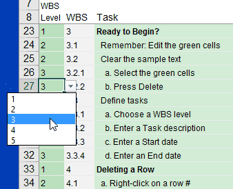
WBS Numbering via Drop-Down
Unlike the free version (and older pro versions), you will not need to copy and paste different WBS formulas for different WBS levels.
For fellow Excel fans: If you are curious about how the mega-formula for the WBS numbering works, you can learn some of the techniques via an article I wrote about various text manipulation formulas. Also, the indenting of the task description is controlled using Conditional Formatting and custom Number formats such as "_s_s_s_s@" to format the text with leading spaces.
2. Multiple Ways to Define Task Dates and Durations
The biggest change in version 4.0 had to do with how you define each task's start and end date. Instead of copying formulas from a set of template rows or cells to define tasks in different ways, you just enter your data in the appropriate input columns.
Watch the Video for Version 5.0
Ultimately, a task needs to have a start date and an end date. You can arrive at those dates in a lot of different ways, depending on whether you want to enter dates manually, enter a duration instead of a date, or whether you want to create dependencies between tasks using Excel formulas.
Now, all you need to do is enter a combination of two inputs. For example, this could be the Start date and End date, or the Start date and number of Work Days. The worksheet has separate columns for the calculated start & end dates. These calculated Start and End dates are what the spreadsheet uses to display the chart.
The downside to this new way of defining tasks is that there are quite a few input columns as well as the calculated columns. However, after you are done defining your tasks, you could hide some or all of the columns you don't need to see.
Tip: In addition to hiding columns to condense the input section of the worksheet, you can use the Arial Narrow font and then make the columns narrower.
Update 12/1/2021: There is now a new Lead/Lag column hidden right after the Predecessors columns. Using this optional column will make the task start X work days after (Lead) or before (Lag) the end date of the predecessor. Enter a positive value for Lead or a negative value for Lag. This column only works in combination with the Predecessors column.
3. Compatibility with Desktop, Mobile and Excel Online
Many of the design aspects of Version 5.0 have to do with making the spreadsheet compatible with Excel Online and Excel Mobile without having to use different versions of the file for different versions of Excel. The spreadsheet uses some features of Excel that are not available in Excel Online such as cross-hatching for displaying Actual vs. Planned - but the spreadsheet also includes a way to make this work in Excel Online (see the help and labels and notes within the spreadsheet).
Questions?
If you have questions about Gantt Chart Pro, please first watch the videos available on the web page, then check the Help worksheet, and then check the FAQ post. If you still can't find the answer to your question, you can contact me.
Q. Why are there two sets of Start/End dates?
The input columns allow you to quickly decide whether to enter dates and/or durations. However, the Gantt chart needs to reference a single column for all Start Dates and a single column for all End Dates. So, the calculated columns use formulas to calculate the dates based on which combination of inputs you choose, and the Gantt chart references these calculated columns.
When printing or presenting, it is better to hide the input columns instead of the calculated columns, because the calculated columns show ALL dates and durations while the inputs may or may not be used. For example, you might define a task by entering a Predecessor and a duration in Days, which means the inputs for Start date and End date are left blank.
Q. Is there any reason to use the older version(s)?
I don't think so, unless you are using an old version of Excel, or you prefer the older designs. However, the older versions will not be updated or supported.
Q. Why are some videos still showing the older versions?
Some older videos are still lingering on Youtube and elsewhere, and for the most part these older videos are still mostly applicable to the new version. See the Gantt Chart Pro page for the most recent videos.
Q. What happens if I enter more than two values to define task durations?
Avoid doing that. If you enter a Start Date and an End Date AND the number of Work Days, then you won't know which of the 3 values were used to calculate the Start and End dates used in the chart.
Q. What is happening when I enter End Date and Work Days as the inputs?
The Start date is calculated to be the number of work days PRIOR to the End date you entered. You might use this for a task that needs to start 5 days prior to the completion of some other task. The End date could be a simple Excel formula that references the end date of the other task.
Q. How do I work backwards from a known project end date, using dependencies?
Version 5.0 allows you to define a task using an End Date and the Duration (in days or work days). You'll just need to enter a formula in the End Date input column such as this one: =WORKDAY.INTL(successor_start_date,-1,weekend,holidays). See the Help worksheet for examples of using formulas to create task dependencies.
Q. What are the little green triangles in some of the cells?
The green triangles are due to the "Error Checking" feature in Excel. Most of the time they aren't actually errors. They may be warnings such as "Number stored as text" or "Inconsistent Formula" or "Unprotected Formula," all of which may be intentional on the part of the user or template designer (such as the WBS numbering purposefully entered as text).
To get rid of the green triangles, you can either choose the "Ignore Error" option every time they show up, or you can go to "Error Checking Options" to turn off some of the various types of warnings.
Q. Will the BONUS files be updated, too?
Perhaps. I've updated the Google Sheets version to 5.0, and will eventually update the other bonus files. However, I do not have a schedule for when that might happen.
Q. How do I show the overall % Complete for the entire project?
The latest update (5.0.1) includes a cell above the % Done column showing the progress for the entire project. If you aren't using the latest version and you want to add this formula to your spreadsheet, you can use the following formula (this requires Excel 2013 or later because of the ISFORMULA function). Note that this formula allows you to ignore the cells in the progress_range that contain formulas, such as if you are calculating the % Done for summary tasks (your overall % Done should not double count the summary tasks rows).
=SUMPRODUCT(workdays_range,progress_range,1*NOT(ISFORMULA(progress_range)))/SUMPRODUCT(workdays_range,1*NOT(ISFORMULA(progress_range)))


Comments
Hi Jon,
This is so Pro! I love it.
Just quick question: With reading all the helps and Q&A, could you quickly tell me what is the major thing I missed out if I just stay with o365 version, but not the desktop version? I mean, what is the reason why I should not just simply use the o365 version? Thanks!
@Leonard, The main thing that the desktop version does differently is display the gantt chart in greater detail in the weekly/monthly/quarterly views. It uses much narrower columns (and therefore many more columns) which means that in the weekly view you are seeing 7 columns per week, while in the o365 versions there is only one column per week. A cell can only be shaded or not shaded, not partially shaded, so that means that in the week view if a task only lasts a single day, it will still highlight the entire cell for the given week. So, the desktop version provides a bit more visual accuracy in the weekly/monthly views than the o365 version. Otherwise, they are mostly the same. The o365 version is probably the best one to use because it is more compatible with Excel Online and Mobile Excel and it only has that one main limitation. I’ll probably end up making the o365 version the one main version and only provide some of the older files and what is now called the ‘desktop version’ as optional downloads.
Hi
Although I have one question I just wanted to say what a fabulous piece of work!
I’m currently using the ‘gantt_chart_v4-0 file’ and I want to be able to see what week my process is in even though my work is daily.
Like Week 22: 25 May – 31 May tucked underneath or above.
Best Regards,
Pao
Not sure I’m following, but you could use a function like WEEKNUM. I don’t think creating pop-up info with a formula is possible (at least not without vba). See the Excel Consulting for an Excel consultant recommendation to help you customize your spreadsheet.
Problem with display “Weekly” and “Monthly”
When I select the display “Weekly” or “Monthly” it does not work.
It appears this:
Display “Weekly”= 00’yy – 00’yy
Display “Monthly” = 00 – 00
I have the impression that the problem comes when I save the file on my computer.
Thanks for yor help
The Gantt Chart spreadsheets are designed for English language settings. If you are not using English language settings, the format codes may not work. You’ll need to update format codes in formatting and in formulas based on your language settings, or if purchased within 60 days, you can request a refund. Thank you.
Hi
I’ve tried asking this before, no answer yet. The Start date column P font size is set as Arial 8 – if I try to change it I cannot. In the font box on the ribbon it will look like font size 10,12,14 or whatever but the actual font size seen is absolutely minute and doesn’t change. How can I change this please. If this is not where I am likely to get an answer, who do I need to ask or email, looking forward to hopefully getting an answer.
@Billy … those cells probably have the “Shrink to Fit” option turned out which ensures that the date fits within the cell rather than showing ######. You can turn that off by going to Format Cells > Alignment tab. You’d then need to change the column width. Or, just keep the Shrink to Fit option on and increase the column width so that the date will fit with the larger font size.
Hi Jon,
How can I create recurring tasks in the “gantt-chart_v5-0_advanced”?
Thanks. Regards, – Ton –
@Ton … that version isn’t designed for recurring tasks unless each task with a start/end date is on a separate row. If you defined your own set of formulas in a header row, it would be possible to set up some type of recurring task display, but if you need help with that type of customization, you’d need to contact a consultant like ExcelRescue.net.
Hi all using the chart and i have to say how user friendly it is, can i ask is there a way of extending what you see so ill try and explain, when you enter a duration you can see up to eight weeks, my project i need to see at least 26 weeks can someone help
See this article for a link to a video showing how to add more columns:
https://www.vertex42.com/blog/help/gantt-chart-help/gantt-chart-support.html#columns
Hi All,
I noticed that for the Gantt Chart v5 for Google Sheets, the cell colouring scheme for weekends and holidays has changed. It appears that all days (weekdays and non-holidays) are now coloured the same colour as weekends and holidays (grey shade). Is it possible Google Sheets pushed out a version that broke this feature?
BTW – I love this product. Keep up the great work!
Thanks,
Randy
Randy, I’ve checked the original templates and they appear to be fine. You might check the Help&Settings worksheet to make sure the weekend option is set correctly (cell C66).
Hi, your “dateformat_wm” in line 10 doesn’t work. results displayed is “Sep YYYY – Nov YYYY” rather than “Sep 2022 – Nov 2022”
can you check that ?
thanks
If you aren’t using English language settings then you’ll need to use a format code appropriate for your language settings. Y is for “Year”, J is for “Jahre”, A is for “Año”, etc. There is a setting in the Help&Settings worksheet for updating this format (the cell that “dateformat_wm” refers to).
I want to change the time period breakdown to months and years rather than days and weeks since I have a long-lasting project and the days and weeks are indefinite at this point. How might I do that?
The Pro version includes a way to change the view to daily/weekly/monthly/quarterly.
In your video where you show how to build a Gantt chart in Excel https://www.youtube.com/watch?v=un8j6QqpYa0, could you show us how to show a task being late to start in red? I love this video but can’t figure out the formula for showing a task that is overdue to start and finish. Thank you in advance!
If you want to have the entire bar turn red if the end date of the task is before today, then you could create a duplicate CF rule (duplicate the one that creates the bars) and add a condition to it like =AND(enddate
Hi
After me working on the fully licensed version and circulate it with the team and 3rd party, that will allow them to received the fully licensed version right. Which may allow them to use the same file to create their scheduled, which will provide them with fill access. What security I have to restrict the receivers to have only the features equivalent to the free version.
There are no security features other than what Excel or Google Sheets provides. It’s up to the purchaser to inform the users to not share the file outside your specific project/team.