This article is dedicated to the various ways that you can use Circular References in Excel on purpose, rather than just as an error signal. I'll share some examples of animated models without VBA, then explain some of the basic building blocks for working with circular references.
IMPORTANT: To USE circular references on purpose, you need to Enable Iterative Calculation. If you set the Maximum Iteration to 1, then you can use F9 to step through each iteration. This can be used for animation or just to watch your model solve one step at a time.
- Examples You Can Download
- Create a Basic Counter
- Use a Checkbox as a Start/Reset Trigger
- Build a Growing Array
- Create a Timer
- Jacobi Updates (make new, replace old with new)
- Gauss-Seidel Updates (update in-place)
- Build in a Loop
- Left-to-Right, Top-to-Bottom
Examples You Can Download
Before diving into the details, you may want to check out these 4 examples:
Example 1: Dice Rolling Simulation
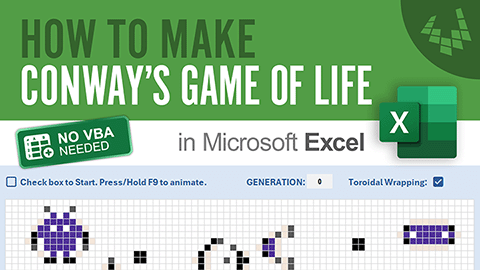
Example 2: Conway's Game of Life
Example 3: Four-Bar Linkage Animation
Example 4: Heat Transfer Simulation
Create a Basic Counter or Iterator
To get started, we will make a Counter that adds 1 or some other increment value each time you press F9.
In cell B1, enter =B1+1. It's as simple as that! B1 is adding 1 to itself each time you press F9.
You can of course add some other increment value in place of 1, such as 0.25 or 0.5 or 10, etc.
IMPORTANT: If you get the circular reference warning/error message, go to File > Options > Formulas and check the "Enable Iterative Calculations" box, and set Maximum Iterations to 1.
Also note that if you are relying on the worksheet adding only a single step each time you press F9, then make sure you aren't using Data Tables or other features that cause Excel to perform additional iterative calculations.
Use a Checkbox as a Start (or Reset) Trigger
Every time I've built a model based on this type of iteration, I've wanted a way to Start and Reset the simulation, animation, etc.
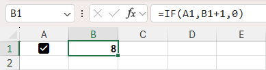
An easy way to do that is to add a Checkbox into cell A1 (via Insert > Checkbox) and modify your Counter formula in cell B1 to be =IF(A1,B1+1,0). This means "If the checkbox in cell A1 is checked (i.e. TRUE), the add one to B1, otherwise make it 0"
Build a Growing Array
The Dice Rolling simulation above shows how you can store random values in a growing array.
To simulate rolling a 6-sided die, we use =RANDBETWEEN(1,6). Put that formula into cell C1.
Keep your checkbox in cell A1 and your Iterator in cell B1.
In cell D1, enter =IF(A1,VSTACK(D1#,C1),C1)
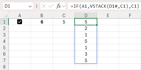
When you click on your checkbox and press F9, you should see the array in cell D1 start growing.
Why is this method interesting? Because normally if you make an array of random numbers using RANDBETWEEN, the numbers will change every time the worksheet recalculates. Yes, you could generate a set of numbers and then paste just those values somewhere, but for this case we are generating a growing array of newly generated random numbers that will remain as-is until we restart the simulation.
Create a Timer
The goal here is to create a functioning timer that keeps track of the amount of real time since the start of a simulation. It will update each time you press F9, and will be reset when you uncheck the box in A2.
For this type of timer, we need to use the concept of "latching". We want to capture the timestamp ONCE, only immediately after the checkbox is first checked.
When the checkbox is checked, we can use the NOW() function to store the current timestamp.
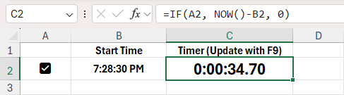
A2 contains a checkbox.
B2 will now represent our Start Time. In B2, enter =IF(A2, IF(B2="",NOW(),B2), "").
C2 =IF(A2, NOW()-B2, 0)
C2 is the time difference between NOW() and our starting timestamp that was stored in B2. You can format C2 using the number format "00:00:00.000". Although times in Excel are not supposed to be accurate to the millisecond, Excel seems to do pretty well with 20ms increments.
How does this work? First, we start out with B2="". Immediately after the checkbox is checked, B1 is still blank, but the formula will use NOW() to return the current time stamp. Every subsequent recalculation, B1 is no longer blank, so it will continue to return the value in B1 (the original time stamp). This is called an "Edge-triggered capture" and we are "latching the start time".
Elapsed Time can be calculated in cell C2 as =IF(checked, NOW()-B2, 0)
Jacobi-style Array Updates
A Jacobi-style update or iteration might be summarized as "use old, replace with new."
For this type of update, we might have an array, such as a Sudoku puzzle, Game of Life map, or a matrix representing a system of linear equations.
We perform whatever calculations are needed and create a new array (typically of the same size). Then, using a circular reference we replace the old array with the new array. Then those calculations are repeated until some type of convergence level is achieved (or a specific number of steps).
For this type of simulation, you would typically need 3 versions of your array. The first is a SEED array, containing the starting values. The second is your CURRENT array. The third is your calculated NEW array.
The formula for the CURRENT array is =IF(started,_new,_seed).
The SEED array is not necessary if you always start with the same initial values, or it could represent your current best guess at the solution. Your _seed array might just be an array the size of _new that is all 0s or 1s.
Gauss-Seidel Updates
A Gauss-Seidel update might be described as "update in place, using new values immediately." Although for this type of update, we are typically talking about a matrix or an array, our Counter at the beginning of the article is a extremely simple example.
Another very simple 1D example might be a sequence that starts at an increasing larger number each step such as B2=IF(started,SEQUENCE(10,,B2+1),0)
A good example of a 2D grid update is the Steady-State Heat Transfer simulation shown in the list of examples above. Here we can actually see a "Heat Map" used for real heat!
Minimum Distance Along a Path
One type of problem that comes up in Excel Esport challenges is solving a minimum distance along a path. This can be done using circular references and a Gauss-Seidel Update. It is an example of a non-rectangular "in-place iterative convergence solution."
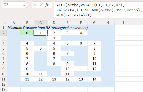
In this example, we are calculating the minimum distance to travel from cell B2 to other cells, following a path (avoiding the blue walls). We start with cell B2 containing a fixed value of 0. Enter the following formula into cell C2:
C2=LET(ortho,VSTACK(C1,C3,B2,D2),validate,IF(ISBLANK(ortho),9999,ortho),MIN(validate)+1).
Then copy that cell to the other locations. After a few iterations, we have the solution.
Build in a Loop
If you don't want to your simulation running away from you, or you want to put your simulation into a loop, then you can define a period for your loop.
Returning to example 1, let's add a value into cell D1 to represent a Period or Total Frames in our loop, such as 5 steps, so D1=5.
Then in cell B1 enter =IF(A1,1+MOD(B1,D1),0)
This will result in cell B1 having this pattern as you press F9: 1,2,3,4,5,1,2,3,4,5,...
I could have used something like this for my Four-Bar Linkage model where the crank angle varies between 0 and 360 degrees over time. However, the model already uses SIN and COS for the angle which results in the same result for 0 degrees as for 360 or 720 degrees. So, MOD was not needed.
Left-to-Right, Top-to-Bottom
One important thing to remember when working with purposeful circular reference calculations is that Excel evaluates the spreadsheet left-to-right, top-to-bottom each iteration until values converge.
If you experience some weird behavior with your model, especially as you are stepping one iteration at a time, it could very likely be a result of forgetting about the left-to-right, top-to-bottom sequence.
Conclusion
There are likely many or even infinite ways of using circular references. These are just some of the examples and building blocks that I have found in my own exploration of Excel. Hope you enjoyed this article.


Comments