SUMIF, SUMIFS, COUNTIF, and COUNTIFS are extremely useful and powerful for data analysis. If there was an Excel Function Hall of Fame, this family of functions ought to be included. In this article, I'll demonstrate a bunch of different ways to use these functions, focusing mainly on all the different criteria types.

The SUMIF and COUNTIF functions allow you to conditionally sum or count cells based on a single condition, and are compatible with almost all versions of Excel:
=SUMIF(criteria_range, criteria, sum_range)
=COUNTIF(criteria_range, criteria)
The SUMIFS and COUNTIFS functions allow you to use multiple criteria, but are only available beginning with Excel 2007:
=SUMIFS(sum_range, criteria_range1, criteria1, criteria_range2, criteria2,...)
=COUNTIFS(criteria_range1, criteria1, criteria_range2, criteria2,...)
AVERAGEIF and AVERAGEIFS are also part of this family of functions and have the same syntax as SUMIF and SUMIFS.
This Article (bookmarks):
1) SUMIF and COUNTIF Examples
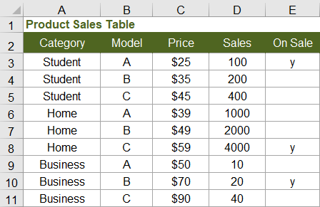
We'll start off by using a product sales table to demonstrate a few different SUMIF and COUNTIF formulas. I've listed a few of these examples below. To see these formulas in action and try them out yourself, you can download the example file below:
Download the Example File (SumIf-CountIf.xlsx)
Criteria are Text Values
Example: Sum of Sales where Category equals "student"
=SUMIF(category_range,"student",sales_range)
NOTE This formula will also match "Student" because the SUMIF family of functions are not case-sensitive. You can use wildcard characters within the text string, such as "?s*" to match values where the second letter is s.
Not Equal To (<>)
Example: Sum of Sales where Model is NOT equal to "B"
=SUMIF(model_range,"<>B",sales_range)
Example: Sum of Sales where Category does NOT contain the letter "u"
=SUMIF(category_range,"<>*u*",sales_range)
Criteria is an Alphabetical Text Comparison
Example: Sum of Sales where Model is less than "C"
=SUMIF(model_range,"<C",sales_range)
Criteria is a Numeric Comparison
Example: Number of products priced over $40
=COUNTIF(price_range,">40")
NOTE When using numeric criteria, COUNTIF and SUMIF ignore text values. Numeric date values can be an exception to that (see below for date comparisons).
Criteria matches Blank Cells or Empty Cells
Example: Count of products where On Sale is blank
=COUNTIF(on_sale_range,"")
Criteria matches Non-Blank Cells
Example: Number of products on sale (where On Sale is not blank)
=COUNTIF(on_sale_range,"<>")
Criteria includes a Cell Reference
Example: Sum of Sales where Price is greater than the value in cell H3
=SUMIF(price_range,">"&H3,sales_range)
Criteria is In Another Cell
Example: Sum of Sales using the criteria defined in cell K9
=SUMIF(criteria_range,K9,sales_range)
NOTE This technique is useful when you want to allow the user to choose or enter different criteria or search strings.
The cell K9 could contain a value like "student" or "40" or a criteria string such as ">40" or "<>student"
Multiple Criteria
Example: Sum of Sales where Category = "student" AND Price > 30
=SUMIFS(sales_range,category_range,"student",price_range,">30")
Example: SUMIFS between two dates
=SUMIFS(sum_range,date_range,">=1/1/2017",date_range,"<1/31/2017")
NOTE The SUMIFS, COUNTIFS, and AVERAGEIFS functions are used for multiple AND conditions. Formulas for OR conditions are a bit more tricky (see below).
2) Using Dates as Criteria
When using dates as criteria for the COUNTIF and SUMIF functions, Excel does some interesting things, depending on whether you are using "=" or "<" as the criteria and whether the dates in the criteria range are stored as numeric date values or text values.
Remember: Date values are stored in Excel as sequential numbers starting with 1 for 1/1/1900. The cell formatting may display the date in different ways, but COUNTIF and SUMIF comparisons are based on the value stored in the cell, not the way a cell is formatted. That is a good, because we normally want to compare dates and numbers without having to worry about how they are formatted.
Criteria is a Date
=COUNTIF(criteria_range,"=3/1/17")
When using criteria such as "=3/1/17" or "Mar 1, 2017", Excel will recognize the criteria as a date and will count all date values in the criteria_range matching that date. Excel will ALSO count recognized dates stored as text values in the criteria_range, such as "March 1, 2017" and "3/1/2017" (but not "March 1st, 2017" because Excel doesn't recognize it as a date).
Criteria is Greater or Less than a Date
=COUNTIF(criteria_range,">3/1/17")
When using <, >, <=, or >=, Excel still recognizes the criteria as a date, but it does not convert text values in the criteria_range to date values.
Comparison to TODAY
You can use the TODAY function to make comparisons based on the current date, like this:
=SUMIF(date_range,"<"&TODAY(),sum_range)
3) SUMIFS Example: Income and Expense Report
SUMIFS is very useful in account registers, budgeting, and money management spreadsheets for summarizing expenses by category and between two dates.
The SUMIFS example below sums the Amount column with 3 criteria: (1) the Category matches "Fuel", (2) the Date is greater than or equal to the start date, and (3) the Date is less than or equal to the end date.
=SUMIFS(amount_range, category_range, "Fuel", date_range, ">=1/1/2018", date_range, "<=1/31/2018")
The following screenshot shows an example from the download file:

4) SUMIF and COUNTIF Between Two Numbers (1 < x < 4)
COUNTIFS and SUMIFS can easily handle a condition such as 1 < x < 4 (which means x > 1 AND x < 4). However, if you are trying to make a spreadsheet compatible with older versions of Excel, you can use COUNTIF or SUMIF by subtracting the results of the condition x <= 1 from the results of the condition x < 4.
| Condition | Formula using COUNTIFS |
|---|---|
| 1 < x < 4 | =COUNTIFS(range,">1",range,"<4") |
| Condition | Formula using only COUNTIF |
| 1 < x < 4 | =COUNTIF(range,"<4") - COUNTIF(range,"<=1") |
| 1 <= x < 4 | =COUNTIF(range,"<4") - COUNTIF(range,"<1") |
| 1 < x <= 4 | =COUNTIF(range,"<=4") - COUNTIF(range,"<=1") |
| 1 <= x <= 4 | =COUNTIF(range,"<=4") - COUNTIF(range,"<1") |
A common need for these formulas is to sum values between two dates. Remember that date values are stored as numbers.
Example: SUMIF between two dates ( 1/1/2017 <= date <= 1/31/2017 )
=SUMIF(sum_range,date_range,"<=1/31/2017")-SUMIF(sum_range,date_range,"<1/1/2017")
5) SUMIF and COUNTIF with OR Conditions
COUNTIFS and SUMIFS handle multiple AND conditions, but OR conditions such as X<2 OR X>3 are usually easier to handle by evaluating each condition separately and then adding the results. The two formulas below do essentially the same thing.
| Condition | Formula |
|---|---|
| x < 2 or 3 < x | =COUNTIF(range,"<2") + COUNTIF(range,">3") |
| x < 2 or 3 < x | =SUM(COUNTIF(range,{"<2",">3"})) |
To avoid double-counting cells, the conditions must not overlap. For example, the condition "=*e*" would overlap with the condition "=yes". The condition "<40" would overlap with the condition ">20". If the conditions overlap, you may end up counting or adding a value twice. If there is a possibility of conditions overlapping, then you may need to use a SUMPRODUCT formula as explained below.
Use SUMPRODUCT for overlapping OR conditions
The key to avoid double-counting is to recognize that FALSE+FALSE=0 and TRUE+FALSE=1 and TRUE+TRUE=2. This means that for a logical OR condition to be true, we can check whether the sum of two or more conditions is > 0.
Sum of Sales where Model is equal to A or B.
=SUMPRODUCT(sales,1*( ((model="A")+(model="B"))>0 ))
Sum of Sales where Model = "A" or Price > 45
=SUMPRODUCT(sales,1*( ((model="A")+(price>45))>0 ))
6) Case-Sensitive SUMIF and COUNTIF
The SUMIF family does not have a case-sensitive option, so we need to resort back to using array formulas or SUMPRODUCT. The FIND and EXACT functions both provide a way to do case-sensitive matches.
Sum of Sales where Category exactly matches "student" (case-sensitive)
=SUMPRODUCT(sales,1*EXACT(category,"student"))
Sum of Sales where Category contains "Stu" (case-sensitive)
=SUMPRODUCT(sales,1*ISNUMBER(FIND("Stu",category)))
7) MAXIF or MINIF Formula
MAXIFS and MINIFS are new Excel functions available in the latest releases (Excel for Microsoft 365, Excel 2019). Their syntax is similar to SUMIFS, allowing you to use multiple criteria.
Older versions of Excel do not have the MAXIFS or MINIFS functions, but you can use an array formula like this (remember to press Ctrl+Shift+Enter):
Example: Find the maximum Price where Model = "A"
(array formula) =MAX(IF(model_range="A",price_range,""))
8) Summary of Different Criteria Types
| CRITERIA TYPE | EXAMPLE | MATCHES ... |
|---|---|---|
| Text Value | "yes" or "=yes" | "yes" or "Yes" (not case-sensitive), the equal sign is optional |
| Text Value with Wildcards | "=?s*" | text values where the second letter is "s" or "S" |
| Alphabetical Text Comparison | "<C" | text values alphabetically less than "C" |
| Equal to a Numeric Value | 20 or "=20" | numeric values equal to 20 |
| Less than or Equal to | "<=20" | numeric values less than or equal to 20 |
| Greater than or Equal to | ">=20" | numeric values greater than or equal to 20 |
| Not Equal to | "<>0" | values not equal to the value 0 |
| Non-Blank | "<>" | values that are not blank (formulas returning "" are not blank) |
| Blank or Empty | "" | values that are blank and formulas that return "" |
| Equal to a Cell Value | A42 or "="&A42 | values equal to the value in cell A42 |
| Comparison to a Cell Value | ">"&A42 | values greater than the value in cell A42 |
| Equal to a Date | "=3/1/17" | date values equal to 3/1/17 as well as text values such as "3/1/17" or "Mar 1, 2017" |
| < or > a Date | ">1/1/2017" | date values greater than 1/1/2017 (text values are ignored) |
Some criteria, such as case-sensitive matches, may only be possible with array formulas or SUMPRODUCT.
You don't use the functions AND, NOT, OR, ISBLANK, ISNUMBER, ISERROR, or other similar functions as criteria for SUMIF and COUNTIF. However, you can use these functions within a SUMPRODUCT formula (but that isn't within the scope of this article).
9) Other Notes
- Comparisons are based on the value stored in the cell, not on how the cell is formatted.
- Error values in both the sum_range and criteria_range are ignored.
- SUMIFS and COUNTIFS formulas are generally faster than their SUMPRODUCT or array formula counterparts.
- The sum_range and criteria_range arguments can be references (e.g. A2:A42), named ranges or formulas that return a range (such as INDEX, OFFSET, or INDIRECT).
- Normally, you'll want the sum_range and criteria_range to be the same length. See the documentation on the Microsoft sites (referenced below) for information about what happens when the sum_range and criteria_range are not the same length.
- The COUNTIF and SUMIF criteria can be a range (e.g. A2:A3) if you enter the formula as an array formula using Ctrl+Shift+Enter.
- The COUNTIF and SUMIF criteria can be a list such as {">1","<4"}, but functions return an array containing results for the separate conditions, not a sum of both conditions (it is not the same as COUNTIFS or SUMIFS).
Some Templates that Use SUMIF
- Invoice Tracker - Uses SUMIF to create an Aging table that shows unpaid invoices past 30 days, 60 days, etc.
- Account Register - Uses a cumulative SUMIF formula to show the current account balance within the register.
- Weekly Money Manager - Uses SUMIF to show actual spending within a budget report.
- Checkbook Register - Uses SUMIF to show the current cleared balance based on whether the reconcile column contains "r" or "c".
References
- Spreadsheet Tips Workbook - vertex42.com - by Jon Wittwer and Brent Weight
- SUMIF Function - support.office.com - The official documentation of the SUMIF function.
- SUMIFS Function - support.office.com - The official documentation of the SUMIFS function.
- COUNTIF Function - support.office.com - The official documentation of the COUNTIF function.
- COUNTIFS Function - support.office.com - The official documentation of the COUNTIFS function.
- SUMIFS With Multiple Criteria and OR Logic - at exceljet.net - Describes how the function works when you use an array for the criteria such as {"=A","=B"}.


Comments
nice sir
Hi
Kindly assist me to count ‘AA’, ‘AB’,’AC and ‘AD’ from ‘X’, ‘Y’ and ‘Z’.
Total AA, AB, AC and AD is 2500 from X, Y and Z
Regards
@Saad, I’m afraid I don’t know what you mean. Are you referring to AA, AB, X, Y, etc as column labels? If you can be more specific, that would help.
Row A Row B
07:00:00 1
07:02:00 2
Result 07:00:00 3
How to calculate
@Manju … You would need to provide more information. Please ask general questions like this via an Excel forum.
I’m looking at the Money Management Template 2.1 and I see you made extensive use of the offset command in the sum command and was wonder why. For example in the balance column, SUM(M4,J5-I5) seems to work just as well as your =SUM(OFFSET(M5,-1,0),J5,-I5)
@Randy … to make it robust to row deletion and sorting.
Jon,
I am try to create a spreadsheet that tracks round counts through a rifle. Similar to a running balance sheet except I am tracking over 100 rifles and need to keep each rifle on its own row and all rifles on one sheet. I am wanting it to show previous round count, new rounds shot(entered data) and then new balance or number of rounds shot. The only data that I want to enter is the number of new rounds shot that will update the previous balance along with the new balance. I keep getting a circular error. I understand why I am getting that error message but cannot figure out the formula that will give me previous and new balance on the same line. Thanks in-advance for your help!
@Steve, are you wanting to enter a new row every time that you fire shots from the rifle? Or do you just want to update the total and maintain 100 rows? If it’s the first case, you could use something very similar to the Money Management Template where each rifle is an “Account” and your Transactions worksheet could indicate the date and the number of rounds used. The Account Balance column would then keep track of the total for each individual rifle.
Jon,
I am try to create a spreadsheet that tracks round counts through a rifle. Similar to a running balance sheet except I am tracking over 100 rifles and need to keep each rifle on its own row and all rifles on one sheet. I am wanting it to show previous round count, new rounds shot(entered data) and then new balance or number of rounds shot. The only data that I want to enter is the number of new rounds shot that will update the previous balance along with the new balance. I keep getting a circular error. I understand why I am getting that error message but cannot figure out the formula that will give me previous and new balance on the same line. Thanks in-advance for your help!
Hello Sir,
Thank you so much for clearing all these concepts and for helping. It’s pretty helpful for us or as beginners can easily understand.
Thanks®ards,
Dipak Alkari
I have two rows of numbers between 1& 5. I want to count the number of columns where both rows are >=2 AND the total of the 2 rows is >=5. So, 2 & 2 would not be counted, but 2 & 3 would. I cannot add a helper row for the total.
Use helper rows in the creation of a larger formula. This is a case where you may need to use some array formulas with boolean tests. Something like this:
=SUM(1*(( (((1:1>=2)+(2:2>=2))=2) + ((1:1+2:2)>=5) )=2))
Or something like this (because BYCOL allows you to use AND in a way that applies only to one column at a time):
=SUM(1*BYCOL(A1:E2,LAMBDA(col,AND(INDEX(col,1)>=2,INDEX(col,2)>=2,SUM(col)>=5))))
Hello
Thank you for this absolutely amazing comprehensive workbook, really Excel should come with this!